") , i = 1,2, ..., n, where x is the independent variable and y is the dependent variable, a polynomial regression fits data to a model of the following form:
, i = 1,2, ..., n, where x is the independent variable and y is the dependent variable, a polynomial regression fits data to a model of the following form:
For a given dataset , i = 1,2, ..., n, where x is the independent variable and y is the dependent variable, a polynomial regression fits data to a model of the following form:

|
(1) |
|---|
where k is the polynomial order. In Origin, k is a positive number that is less than 10. Parameters are estimated using a weighted least-square method. This method minimizes the sum of the squares of the deviations between the theoretical curve and the experimental points for a range of independent variables. After fitting, the model can be evaluated using hypothesis tests and by plotting residuals.
 is the y-intercept and the parameters
  ,
,  , ... ,
  are called the "partial coefficients" (or "partial slopes").
It can be written in matrix form:
are called the "partial coefficients" (or "partial slopes").
It can be written in matrix form:

|
(2) |
|---|
and
|
|
Assuming that  are independent and identically distributed as normal random variables with
  and
and ![Var[E]=\sigma^2](/origin-help/en/images/Polynomial_Regression_Results/math-5d3cf3883ed3c4d0b917f9fc2e8f776b.png?v=0 "Var[E]=\sigma^2") .
In Order to minimize the
.
In Order to minimize the  with respect to
  , we solve the function:

|
(3) |
|---|
The results  is the least square estimate of the vector B, and it is the solution to the linear equations, which can be expressed as:
^{-1}X^{\prime }Y")
|
(4) |
|---|
where X' is the transpose of X. The predicted value of Y for a given X is:

|
(5) |
|---|
By substituting  into (4), we can and defined matrix
  .
.
![\hat{Y}=[X(X'X)^{-1}X']Y=PY](/origin-help/en/images/Polynomial_Regression_Results/math-9a8d7df1113cf6e1902177ad13919636.png?v=0 "\hat{Y}=[X(X'X)^{-1}X']Y=PY")
|
(6) |
|---|
The residuals is defined as:

|
(7) |
|---|
and the residual sum of squares can be written by:

|
(8) |
|---|
| Note: It is worth noting that the higher order terms in polynomial equation have the greatest effect on the dependent variable. Consequently, models with high order terms (higher than 4) are extremely sensitive to the precision of coefficient values, where small differences in the coefficient values can result in a larges differences in the computed y value. We mention this because, by default, the polynomial fitting results are rounded to 5 decimal places. If you manually plug these reported worksheet values back into the fitted curve, the slight loss of precision that occurs in rounding will have a marked effect on the higher order terms, possibly leading you to conclude wrongly, that your model is faulty. If you wish to perform manual calculations using your best-fit parameter estimates, make sure that you use full-precision values, not rounded values. Note that while Origin may round reported values to 5 decimal places (or other), these values are only for display purposes. Origin always uses full precision (double(8)) in mathematical calculations unless you have specified otherwise. For more information, see Numbers in Origin in the Origin Help file.
Generally speaking, any continuous function can be fitted to a higher order polynomial model. However, higher order terms may not have much practical significance. |
In above section, we assume that there is constant variance in the errors. However, when we fit with the experimental data, we may need to take account of the instrument error (which reflect the accuracy and precision of a measuring instrument) in fitting process. Therefore, the assumption of constant variance in the errors is violated. We need to assume to be normally distributed with nonconstant variance, and the errors act as  , which can be used as weight in fitting. The weight is defined as:

|
|---|
The fitting model is changed into:
![\sum_{i=1}^n w_i (y_i-\hat y_i)^2=\sum_{i=1}^n w_i [y_i-(\hat{\beta _0}+\hat{\beta _1}x_i)]^2](/origin-help/en/images/Polynomial_Regression_Results/math-b91af30efe2f541053551a9080cdf9de.png?v=0 "\sum_{i=1}^n w_i (y_i-\hat y_i)^2=\sum_{i=1}^n w_i [y_i-(\hat{\beta _0}+\hat{\beta _1}x_i)]^2")
|
(9) |
|---|
The weight factors  can be given by three formulas:
The error bar will not be treated as weight in calculation.

|
(10) |
|---|
As for Instrumental weight, the value is inversely proportional to the instrumental errors, so a trial with small errors will have a large weight because it is rather precise than those with larger errors.

|
(11) |
|---|
| Note: the errors as weight should be desiganited as "YError" column in worksheet. |
Fix intercept will set the y-intercept  to a fixed value, meanwhile, the total degree of freedom will be n*=n-1 due to the intercept fixed.
Scale Error with sqrt(Reduced Chi-Sqr) is available when fitting with weight. This option only affects the error on the parameters reported from the fitting process, and does not affect the fitting process or the data in any way.
By default, it is checked, and , which is the variance of  is taken into account for calculating error on the parameters, otherwise variance of will not be taken for error calculation.
Take Covariance Matrix as example:
is taken into account for calculating error on the parameters, otherwise variance of will not be taken for error calculation.
Take Covariance Matrix as example:
Scale Error with sqrt(Reduced Chi-Sqr)
=\sigma^2 (X^{\prime }X)^{-1}")
|
(12) |
|---|---|

|
Do not Scale Error with sqrt(Reduced Chi-Sqr)
=(X'X)^{-1}\,\!")
|
(13) |
|---|
For weighted fitting, ^{-1}\,\!") is used instead of
is used instead of ^{-1}\,\!") .
.

Formula (4)
For each parameter, the standard error can be obtained by:

|
(14) |
|---|
where  is the jth diagonal element of
 ^{-1}") (note that
(note that ^{-1}") is used for weight fitting). The residual standard deviation
is used for weight fitting). The residual standard deviation  (also called "std dev", "standard error of estimate", or "root MSE") is computed as:

|
(15) |
|---|
is an estimate of  , which is variance of
Note: Please read the ANOVA Table for more details about the degree of freedom (df),  . .
|
If the regression assumptions hold, we can perform the t-tests for the regression coefficients with the null hypotheses and the alternative hypotheses:


The t-values can be computed as:

|
(16) |
|---|
With the t-value, we can decide whether or not to reject the corresponding null hypothesis. Usually, for a given Confidence Level for Parameters:  , we can reject
  when
when  . Additionally, the p-value is less than .
The probability that  in the t test is true.
)\,\!")
|
(17) |
|---|
where ") compute the cumulative distribution function of the Student's t distribution at the values |t|, with degree of freedom of error
compute the cumulative distribution function of the Student's t distribution at the values |t|, with degree of freedom of error ") .
.
From the t-value, we can calculate the \times 100\%") Confidence Interval for each parameter by:
Confidence Interval for each parameter by:
}\varepsilon _{\hat \beta _j}\leq \hat \beta _j\leq \hat \beta _j+t_{(\frac \alpha 2,n^{*}-k)}\varepsilon _{\hat \beta _j}")
|
(18) |
|---|
where  and
and  is short for the Upper Confidence Interval and Lower Confidence Interval, respectively.
The Confidence Interval Half Width is:

|
(19) |
|---|
Some fit statistics formulas are summary here:
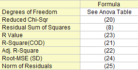
The degree of freedom for (Error) variation. Please refer to the ANOVA table for more details.
|
|
(20) |
|---|
The residual sum of squares, see formula (8).
The goodness of fit can be evaluated by Coefficient of Determination (COD),  , which is given by:

|
(21) |
|---|
The adjusted is used to adjust the value for the degree of freedom. It can be computed as:

|
(22) |
|---|
Then we can compute the R-value, which is simply the square root of :

|
(23) |
|---|
Root Mean Square of the Error, or residual standard deviation, which equals to:

|
(24) |
|---|
Equals to square root of RSS:

|
(25) |
|---|
The ANOVA table of polynomial fitting is:
| df | Sum of Squares | Mean Square | F Value | Prob > F | |
|---|---|---|---|---|---|
| Model | k | 
|

|

|
p-value |
| Error | n* - k | 
|
")
|
||
| Total | n* | 
|
| Note: If intercept is included in the model, n*=n-1. Otherwise, n*=n and the total sum of squares is uncorrected. |
Where the total sum of square, TSS, is:
^2") (corrected) (corrected)
|
(26) |
|---|---|
 (uncorrected) (uncorrected)
|
(27) |
The F value here is a test of whether the fitting model differs significantly from the model y=constant.
Additionally, the p-value, or significance level, is reported with an F-test. We can reject the null hypothesis if the p-value is less than , which means that the fitting model differs significantly from the model y=constant.
If fixing the intercept at a certain value, the p value for F-test is not meaningful, and it is different from that in Polynomial linear regression without the intercept constraint.
To run the lack of fit test, you need to have repeated observations, namely, "replicate data" , so that at least one of the X values is repeated within the dataset, or within multiple datasets when concatenate fit mode is selected.
Notations used for fit with replicates data:
 is the jth measurement made at the ith x-value in the dataset is the jth measurement made at the ith x-value in the dataset |
 is the average of all of the y values at the ith x-value is the average of all of the y values at the ith x-value |
 is the predicted response for the jth measurement made at the ith x-value is the predicted response for the jth measurement made at the ith x-value |
The sum of square in table below is expressed by:
^2")
|
|---|
^2")
|
^2")
|
The Lack of fit table of linear fitting is:
| DF | Sum of Squares | Mean Square | F Value | Prob > F | |
|---|---|---|---|---|---|
| Lack of Fit | c-k-1 | LFSS | MSLF = LFSS / (c - k - 1) | MSLF / MSPE | p-value |
| Pure Error | n - c | PESS | MSPE = PESS / (n - c) | ||
| Error | n*-k | RSS |
| Note: If intercept is included in the model, n*=n-1. Otherwise, n*=n and the total sum of squares is uncorrected. If the slope is fixed, c denotes the number of distinct x values. If intercept is fixed, DF for Lack of Fit is c-k. |
The covariance matrix for the multiple linear regression can be calculated as
=\sigma ^2(X^{\prime }X)^{-1}")
|
(28) |
|---|
In particular, the covariance matrix for the simple linear regression can be calculated as
 & Cov(\beta _0,\beta _1)\\
Cov(\beta _1,\beta _0) & Cov(\beta _1,\beta _1)
\end{pmatrix}=\sigma ^2\frac 1{SXX}\begin{pmatrix} \sum \frac{x_i^2}n & -\bar x \\-\bar x & 1 \end{pmatrix}")
|
(29) |
|---|
The correlation between any two parameters is:
=\frac{Cov(\beta _i,\beta _j)}{\sqrt{Cov(\beta _i,\beta _i)}\sqrt{Cov(\beta _j,\beta _j)}}")
|
(30) |
|---|
The confidence interval for the fitting function says how good your estimate of the value of the fitting function is at particular values of the independent variables. You can claim with 100 % confidence that the correct value for the fitting function lies within the confidence interval, where is the desired level of confidence. This defined confidence interval for the fitting function is computed as:
![\hat{Y}\pm t_{(\alpha/2,dof)}{\left [\chi^2\mathbf{x}\mathbf{C}\mathbf{x}' \right ]}^{\frac{1}{2}}](/origin-help/en/images/Polynomial_Regression_Results/math-a2cba3c7fb1add639804a63591d529b5.png?v=0 "\hat{Y}\pm t_{(\alpha/2,dof)}{\left [\chi^2\mathbf{x}\mathbf{C}\mathbf{x}' \right ]}^{\frac{1}{2}}")
|
(31) |
|---|
where
![\mathbf{x}=\left [ \frac{\partial y}{\partial \beta_0},\frac{\partial y}{\partial \beta_1},\frac{\partial y}{\partial \beta_2},...,\frac{\partial y}{\partial \beta_k} \right ]](/origin-help/en/images/Polynomial_Regression_Results/math-5a5d1b301c0a94216119e6e490f4e688.png?v=0 "\mathbf{x}=\left [ \frac{\partial y}{\partial \beta_0},\frac{\partial y}{\partial \beta_1},\frac{\partial y}{\partial \beta_2},...,\frac{\partial y}{\partial \beta_k} \right ]")
|
(32) |
|---|
and C is the Covariance Matrix.
The prediction interval for the desired confidence level α is the interval within which 100% of all the experimental points in a series of repeated measurements are expected to fall at particular values of the independent variables. This defined prediction interval for the fitting function is computed as:
![\hat{Y}\pm t_{(\alpha/2,dof)}{\left [\chi^2(1+\mathbf{x}\mathbf{C}\mathbf{x}') \right ]}^{\frac{1}{2}}](/origin-help/en/images/Polynomial_Regression_Results/math-9548b3e4b4bf2ff2b5c83da6ed6ca8b5.png?v=0 "\hat{Y}\pm t_{(\alpha/2,dof)}{\left [\chi^2(1+\mathbf{x}\mathbf{C}\mathbf{x}') \right ]}^{\frac{1}{2}}")
|
(33) |
|---|
Select one residual type among Regular, Standardized, Studentized, Studentized Deleted for Plots.
Scatter plot of residual  vs. indenpendent variable
  , each plot is locate in a seperate graphs.
Scatter plot of residual vs. fitted results 
 vs. sequence number
The Histogram plot of the Residual
Residuals vs. lagged residual }") .
.
A normal probability plot of the residuals can be used to check whether the variance is normally distributed as well. If the resulting plot is approximately linear, we proceed assuming that the error terms are normally distributed. The plot is based on the percentiles versus ordered residual, the percentiles is estimated by
}{(n+\frac{1}{4})}")
where n is the total number of dataset and i is the ith data. Also refer to Probability Plot and Q-Q Plot
 ,
,

 ,
,

 = 0.
= 0.