Origin offers data filters of three data formats, date time, numeric, and text. The data filter could be added, removed, enabled, disabled, or reapplied by button click in the Worksheet Data toolbar and customized with user defined filtering conditions.
You can also apply a data filter to column label row data by switching to Column List View (View: Column List View) and applying a data filter to a List View column. For more information, see Column List View - Applying a Data Filter. |
Once you have added a filter to a column, you can check the filtering status from the color of the filter icon on the column header.
To add or remove a data filter to the one or several columns:
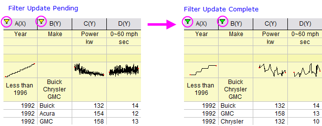
When a data filter is added, it is by default an empty filter, no filtering condition is set. Once filtering conditions are set, the filter is automatically named by the filter condition and the filter icon is fully filled with color green.
Clicking the Add/Remove Data Filter button on a selected column with an applied filter, removes the filter. The same thing is done when you clear a filter from the filter icon menu.
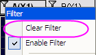
If you want to toggle your filter on or off without losing your filter, just disable the filter (see next).
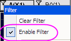
When a data filter is added, it is possible to enable or disable it by either of the following:
or
If multiple columns are selected in the second case, only the data filter of the leftmost selected column will be disabled/enabled.
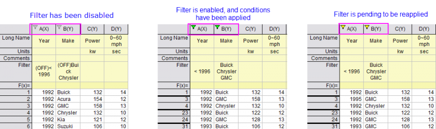
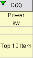
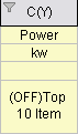
When a data filter is disabled, the filter icon turns to grey, and there is an "off" before the filter name.
If your selected range of columns include both enabled and disabled columns, when you click the ![]() button, all columns will be disabled.
button, all columns will be disabled.
Like MS Excel, when you make changes to filtered data in a worksheet column, you must reapply the filter. When the filter is in need of being reapplied, the filter icon will turn yellow. You can reapply the filter by clicking the Reapply data filter ![]() button on the Worksheet Data toolbar.
button on the Worksheet Data toolbar.
Note: We may introduce LabTalk variables into the filter condition. In general, the filter condition with the variables will be cached after the filter is run. Thus, the result will not change after you click the Reapply Data Filter button wks.runfilter() to reapply filter.
|
By default, when saving a workbook with a Data Connector, imported data are excluded (not saved with the file). If you add a data filter to the workbook, when the file is reopened, the data filter is auto-run after import. If you do not want the data filter to auto-run on import, set @WFI=0. For information on changing the value of a LabTalk system variable, see this FAQ. |
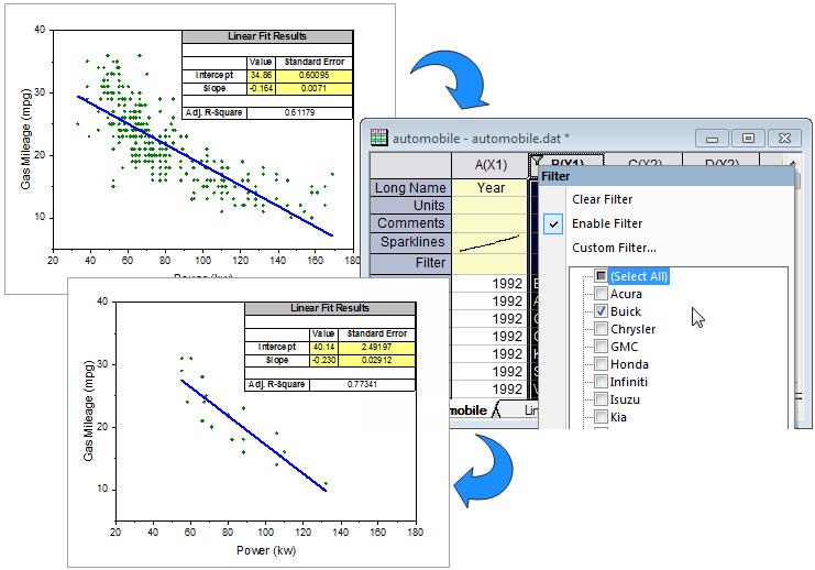
You can copy a data filter from one worksheet column and apply it to other columns. This includes custom filters in which use variables defined in the Before Condition Script panel.
OR,
OR, for numeric column,
Origin will detect the data type and automatically assign one of the three data filters (date, numeric, text) to the corresponding columns. The filtering conditions need to be set when customizing data filters.
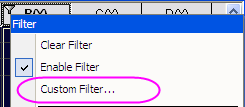
There are two ways to customize a data filter,
or
Once you've added filter conditions, you can double-click on the Filter cell to edit the filter. |
Three general types of filters are supported, grouped by Format:
Available menu options vary by Format. Origin uses the column's Format Properties to determine which menu options to display.
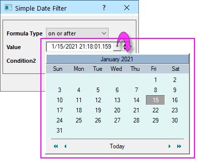
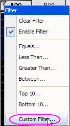
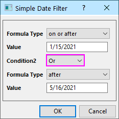
When the column Format = Date, you have the following filtering options:
Clicking Equals, Before or After will open the Simple Date Filter dialog box. Clicking Between provides a simple dialog for setting a date range.
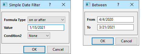
Set the Formula Type, Value and Condition2 or From and To, to filter by date.
The Simple Date Filter Condition2 is used for And/Or filtering. The default state is None but you can set the drop-down to either And or Or and create a second filter condition.
| None | No second filter condition (default). |
|---|---|
| And | Keep rows where the date and time holds true for both query conditions, and hide others. |
| Or | Keep the rows where the date and time holds for either one of the two query conditions, and hide others. |
For more advanced filtering, use the Custom Data Filter dialog, available when you click the Custom Filter menu item at the bottom of the Date filter menu.
Previously, Value, To and From used a standard date-picker control which has been replaced by a simple text field. To revert to the date-picker set system variable @DP = 1. |
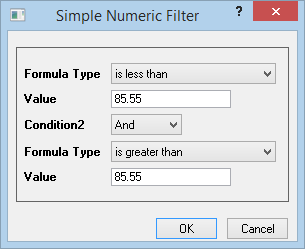
When the column Format = Numeric, you have the following filtering options:
Clicking Equals, Less Than or Greater Than will open the Simple Numeric Filter dialog box. Clicking Between provides a simple dialog for setting a numeric range.
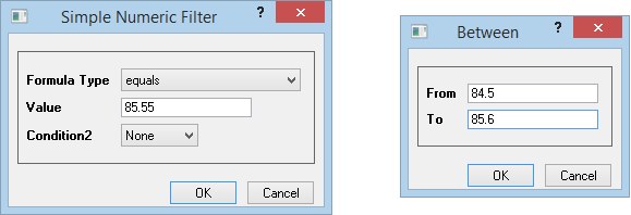
Set the Formula Type, Value and Condition2 or From and To, to filter by number.
The Simple Numeric Filter Condition2 is used for And/Or filtering. The default state is None but you can set the drop-down to either And or Or and create a second filter condition.
| None | No second filter condition (default). |
|---|---|
| And | Keep rows where the numeric condition holds true for both query conditions, and hide others. |
| Or | Keep rows where the numeric condition holds for either one of the two query conditions, and hide others. |
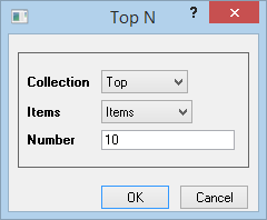
Clicking Top 10 or Bottom 10 opens the the Top N dialog box. Here you can filter out all but the highest or lowest values by number of Items or by Percent.
For more advanced filtering, use the Custom Data Filter dialog, available when you click the Custom Filter menu item at the bottom of the Date filter menu.
The text filter will be applied if the data format of the selected column is Text, Month or Day of Week.
From the quick menu, you can select/deselect the check boxes to show/hide corresponding text entries.
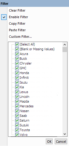
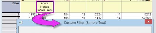
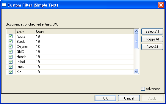
Click the Custom Filter quick menu item to bring up the Custom Filter(Simple Text) dialog.
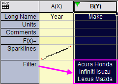
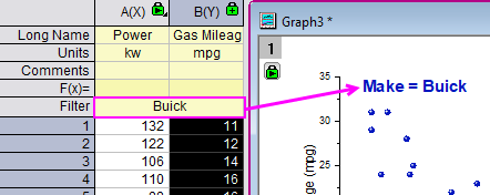
After applying a text filter, the Filter label row will contain a list of the text entries which have not been hidden with the filter. By default, the entries in this cell are separated by a space (" "). The system variable @TFS can be used to switch the separator: 0=Enter, 1=Space, 2=Comma, 3=Semicolon. Another system variable @TFL can be used to set the max number of characters in the text filter label row. By default, this value is 50. The first string and last string will always show in full (sorting is alphabetical); unlisted strings will be shown as "...". For information on these two LabTalk System Variables see the LabTalk System Variable List. |
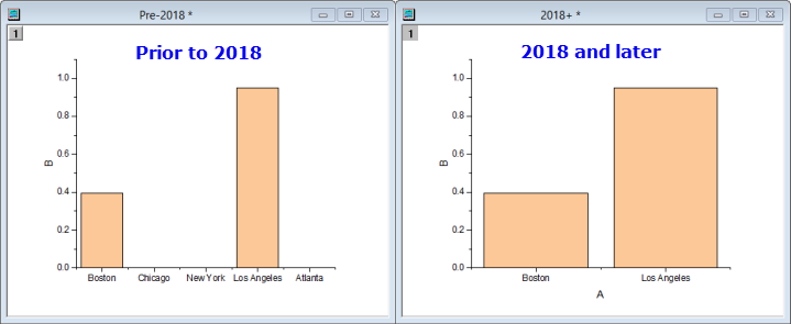
When the X column of a column/bar graph contains text, this text is used to label major ticks, ordered by row index. Prior to Origin 2018, when applying a worksheet data filter, plots registered the vacant ticks and labels of filtered data, though the data points were not plotted. This was changed in Origin 2018 so that ticks associated with filtered data no longer display. This only applies to X columns that contain text and are NOT Set as Categorical. You can restore the pre-2018 behavior using |
Select the Advanced check box to bring up the Custom Filter(Advanced Text) dialog.
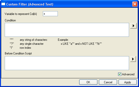
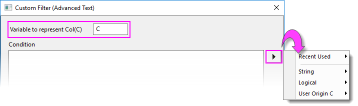
You can use any combination of direct keyboard entry and menu selection to build your expression. The dialog box lists some key elements (wildcard characters, row index) and shows an example expression.
| Example | Description |
| NOT(make="Buick" OR make="Chrysler") | Filter out "Buick" and "Chrysler" |
| !(make="Buick" OR make="Chrysler") | Filter out "Buick" and "Chrysler" |
| !(make="Buick" || make="Chrysler") | Filter out "Buick" and "Chrysler" |
| Symbol | Usage |
| ?(question mark) | Stands for any single character, e.g. "a?c" finds "abc" or "adc" but will not find "abbc" |
| *(asterisk) | Stands for any string of characters, e.g. "abc*e" finds "abcde" or "abcdde" or "abce" |
| ==(two equation marks) | Stands for full match, e.g. x=="a*" finds exactly "a*" but not "abc" |
The following short tutorial will show you how to use the wildcard control for text filter.
|
The Custom Data Filter dialog is used to perform advanced filtering of Date and Numeric data.
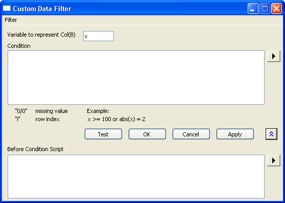
| Test | The rows which meet the filter condition will be highlighted in the original worksheet, these rows will remain after filtering. |
|---|---|
| OK | Apply the change of filter conditions and close the dialog. |
| Cancel | Close the dialog without applying the modification of filter conditions. |
| Apply | Apply the change of filter conditions without closing the dialog. |
For numeric filtering, a few built-in LabTalk functions are not included in the fly-out menu. The following table documents these functions:
| Expression | Usage |
| x.between(x1,x2) | Return the sub range of x between user-input values x1 and x2, equal to x<=x2 && x>=x1. *See note below table. |
| x.top(10,0) | Return the top 10 values of x. |
| x.top(10,1) | Return the top 10% of values of x. |
| x.bottom(10,0) | Return the bottom 10 values of x. |
| x.bottom(10,1) | Return the bottom 10% of values of x. |
| x.top(n,0/1) | Return the top n values of x; when 0 is chosen, n is the number of items, when 1 is chosen, n is the percentage. |
| x.bottom(n,0/1) | Return the bottom n values of x; when 0 is chosen, n is the number of items, when 1 is chosen, n is the percentage. |
* In this expression, x1 and x2 are typically row numbers. If you wish to use variables in this expression, you should not use "x1" and "x2" as they are widely-used system variables and their values may change. Instead, consider using page variables v1...v4.
For Text, Date, and Numeric filters, Origin also supports the function x.count() to count the number of the duplicated data. For example: To keep text data which number is over 3, in the Custom Data Filter dialog you can set: |
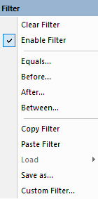
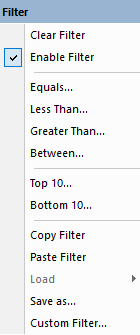
From the Filter menu you can:
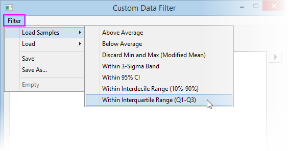
Loaded filters display at the bottom of this menu (if none loaded, reads "Empty").
By default, rows hidden by a filter are ignored in graphing operations. You can change this behavior and include such rows using either of the following:
wks.ignorehidden = 0;
or
| Note: Hidden rows are not ignored in LT scripts and Set Values. |
When you apply a mask and add a data filter on the column data, the masked data is still shown on the column by default. Whether showing the masked data on the column with data filter, that is controlled by the system variable @FBM.
|
In the Recalculate lock icon's context menu for Copy Columns to... and Pivot Table, there are three worksheet filter options. They are used to control whether the results will be affected by further filter changes.
Note: Recalculate Mode of Copy Columns and Pivot Table should be set to Auto or Manual.
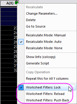
| Worksheet Filters:Lock |
When this option is selected, the result will be locked from data filter condition change of source column(s). So when the filter condition in the source column worksheet is changed, it will not trigger update in the result columns. |
|---|---|
| Worksheet Filters:Reload |
This option is only available when the Worksheet Filter: Lock has been selected already. It reloads the data filter condition from the source column(s) to the result column(s). i.e. after you changed the data filter condition of the source column(s), click this option to trigger the auto update of the locked result column(s), so that the same filter condition applies to result column(s) as well. |
| Worksheet Filters:Push Back |
This option is only available when the Worksheet Filter: Lock has been selected already. It pushes the initial data filter condition back to the source column(s). i.e. after you changed the data filter condition of the source worksheet, click this option and the most recent data filter condition that has been applied from source column(s) to result column(s) will be pushed back to the source worksheet. Note that if you applied a data filter directly to result column(s), it will not be pushed back to source. |
You can add a text label to your graph that combines literal text with the current filter condition. For instance in the following example, we combine literal text "Make =" with a string "%(1, @LF)" to create a dynamic label that changes with the change in filter conditions (i.e. note that for the label to update, the filter cannot be locked). |