 on the dependent variable y. For a given dataset
 ") , the multiple linear regression fits the dataset to the model:
, the multiple linear regression fits the dataset to the model:
Multiple linear regression is an extension of the simple linear regression where multiple independent variables exist. It is used to analyze the effect of more than one independent variable on the dependent variable y. For a given dataset , the multiple linear regression fits the dataset to the model:

|
(1) |
|---|
where  is the y-intercept and the parameters
  ,
,  , ... ,
  are called the partial coefficients.
It can be written in matrix form:
are called the partial coefficients.
It can be written in matrix form:

|
(2) |
|---|
where
|
|
Assuming that  are independent and identically distributed as normal random variables with
  and
and ![Var[E]=\sigma^2](/origin-help/en/images/Multiple_Regression_Results/math-5d3cf3883ed3c4d0b917f9fc2e8f776b.png?v=0 "Var[E]=\sigma^2") .
In Order to minimize the
.
In Order to minimize the  with respect to
  , we solve the function:

|
(3) |
|---|
The results  is the least square estimate of the vector B, and it is the solution to the linear equations, which can be expressed as:
^{-1}X^{\prime }Y")
|
(4) |
|---|
where X' is the transpose of X. The predicted value of Y for a given X is:

|
(5) |
|---|
By substituting  into (4), we can and defined matrix
  .
.
![\hat{Y}=[X(X'X)^{-1}X']Y=PY](/origin-help/en/images/Multiple_Regression_Results/math-9a8d7df1113cf6e1902177ad13919636.png?v=0 "\hat{Y}=[X(X'X)^{-1}X']Y=PY")
|
(6) |
|---|
The residuals is defined as:

|
(7) |
|---|
and the residual sum of squares can be written by:

|
(8) |
|---|
We can give weight to each  in fitting process, the yEr± error column
  is treated as weight
  for each , when yEr± is abscent, should be 1 for all
  .
.
The solution for fitting with weight can be written as:
^{-1}X'WY")
|
(9) |
|---|
where

The error bar will not be treated as weight in calculation.

|
(10) |
|---|

|
(11) |
|---|
Fix intercept will set the y-intercept  to a fixed value, meanwhile, the total degree of freedom will be n*=n-1 due to the intercept fixed.
Scale Error with sqrt(Reduced Chi-Sqr) is available when fitting with weight. This option only affects the error on the parameters reported from the fitting process, and does not affect the fitting process or the data in any way.
By default, it is checked, and  , which is the variance of
  is taken into account for calculating error on the parameters, otherwise, variance of will not be taken into account for error calculation.
Take Covariance Matrix as example:
is taken into account for calculating error on the parameters, otherwise, variance of will not be taken into account for error calculation.
Take Covariance Matrix as example:
Scale Error with sqrt(Reduced Chi-Sqr)
=\sigma^2 (X^{\prime }X)^{-1}")
|
(12) |
|---|---|

|
Do not Scale Error with sqrt(Reduced Chi-Sqr)
=(X'X)^{-1}\,\!")
|
(13) |
|---|
For weighted fitting, ^{-1}\,\!") is used instead of
is used instead of ^{-1}\,\!") .
.

Formula (4)
For each parameter, the standard error can be obtained by:

|
(14) |
|---|
where  is the jth diagonal element of
 ^{-1}") (note that
(note that ^{-1}") is used for weight fitting). The residual standard deviation
is used for weight fitting). The residual standard deviation  (also called "std dev", "standard error of estimate", or "root MSE") is computed as:

|
(15) |
|---|
 is an estimate of
  , which is variance of
| Note: Please read the ANOVA Table for more details about the degree of freedom (df), dfError. |
If the regression assumptions hold, we can perform the t-tests for the regression coefficients with the null hypotheses and the alternative hypotheses:


The t-values can be computed as:

|
(16) |
|---|
With the t-value, we can decide whether or not to reject the corresponding null hypothesis. Usually, for a given Confidence Level for Parameters:  , we can reject
  when
when  . Additionally, the p-value is less than .
The probability that  in the t test is true.
)\,\!")
|
(17) |
|---|
where ") computes the cumulative distribution function of the Student's t distribution at the values |t|, with degree of freedom of error
computes the cumulative distribution function of the Student's t distribution at the values |t|, with degree of freedom of error ") .
.
From the t-value, we can calculate the \times 100\%") Confidence Interval for each parameter by:
Confidence Interval for each parameter by:
}\varepsilon _{\hat \beta _j}\leq \hat \beta _j\leq \hat \beta _j+t_{(\frac \alpha 2,n^{*}-k)}\varepsilon _{\hat \beta _j}")
|
(18) |
|---|
where  and
and  is short for the Upper Confidence Interval and Lower Confidence Interval, respectively.
The Confidence Interval Half Width is:

|
(19) |
|---|
The Variance Inflation Factor is:

|
(20) |
|---|
Where:  is unadjusted coefficient of determination for regression the ith independent variable on the remaining ones.
Some fit statistics formulas are summary here:
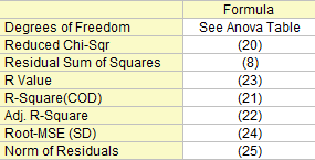
The degree of freedom for (Error) variation. Please refer to the ANOVA table for more details.
|
|
(21) |
|---|
The residual sum of squares, see formula (8).
The goodness of fit can be evaluated by Coefficient of Determination (COD),  , which is given by:

|
(22) |
|---|
The adjusted is used to adjust the value for the degree of freedom. It can be computed as:

|
(23) |
|---|
Then we can compute the R-value, which is simply the square root of :

|
(24) |
|---|
Root Mean Square of the Error, or residual standard deviation, which equals to:

|
(25) |
|---|
Equals to square root of RSS:

|
(26) |
|---|
The ANOVA table of linear fitting is:
| df | Sum of Squares | Mean Square | F Value | Prob > F | |
|---|---|---|---|---|---|
| Model | k | 
|

|

|
p-value |
| Error | n* - k | 
|
")
|
||
| Total | n* | 
|
| Note: If intercept is included in the model, n*=n-1. Otherwise, n*=n and the total sum of squares is uncorrected. |
Where the total sum of square, TSS, is:
^2") (corrected) (corrected)
|
(27) |
|---|---|
 (uncorrected) (uncorrected)
|
The F value here is a test of whether the fitting model differs significantly from the model y=constant.
Additionally, the p-value, or significance level, is reported with an F-test. We can reject the null hypothesis if the p-value is less than , which means that fitting model differs significantly from the model y=constant.
If fixing the intercept at a certain value, the p value for F-test is not meaningful, and it is different from that in multiple linear regression without the intercept constraint.
To run the lack of fit test, you need to have repeated observations, namely, "replicate data" , so that at least one of the X values is repeated within the dataset, or within multiple datasets when concatenate fit mode is selected.
Notations used for fit with replicates data:
 is the jth measurement made at the ith x-value in the data set is the jth measurement made at the ith x-value in the data set |
|---|
 is the average of all of the y values at the ith x-value is the average of all of the y values at the ith x-value |
 is the predicted response for the jth measurement made at the ith x-value is the predicted response for the jth measurement made at the ith x-value |
The sum of square in table below is expressed by:
^2")
|
|---|
^2")
|
^2")
|
The Lack of fit table of linear fitting is:
| DF | Sum of Squares | Mean Square | F Value | Prob > F | |
|---|---|---|---|---|---|
| Lack of Fit | c-k-1 | LFSS | MSLF = LFSS / (c - k - 1) | MSLF / MSPE | p-value |
| Pure Error | n - c | PESS | MSPE = PESS / (n - c) | ||
| Error | n*-k | RSS |
| Note: If intercept is included in the model, n*=n-1. Otherwise, n*=n and the total sum of squares is uncorrected. If the slope is fixed, c denotes the number of distinct x values. If intercept is fixed, DF for Lack of Fit is c-k. |
The covariance matrix for the multiple linear regression can be calculated as
=\sigma ^2(X^{\prime }X)^{-1}")
|
(28) |
|---|
The correlation between any two parameters is:
=\frac{Cov(\beta _i,\beta _j)}{\sqrt{Cov(\beta _i,\beta _i)}\sqrt{Cov(\beta _j,\beta _j)}}")
|
(29) |
|---|
 stands for the Regular Residual
  .
.

|
(30) |
|---|
Also known as internally studentized residual.

|
(31) |
|---|
Also known as externally studentized residual.

|
(32) |
|---|
In the equations for the Studentized and Studentized deleted residuals,  is the ith diagonal element of the matrix :
^{-1}X^{\prime }")
|
(33) |
|---|
 means the variance is calculated based on all points but exclude the ith.
In multiple regression, partial leverage plots can be used to study the relationship between the independent variable and a given dependent variable. In the plot, the partial residual of Y is plotted against the partial residual of X, or the intercept. The partial residual of a certain variable is the regression residual with that variable omitted in the model.
Take the model  for example: the partial leverage plot for
  is created by plotting the regression residual of
  against the residual of
  .
.
Select one residual type among Regular, Standardized, Studentized, Studentized Deleted for Plots.
Scatter plot of residual  vs. indenpendent variable
  , each plot is locate in a seperate graphs.
Scatter plot of residual vs. fitted results  .
.
vs. sequence number
The Histogram plot of the Residual
Residuals vs. lagged residual }") .
.
A normal probability plot of the residuals can be used to check whether the variance is normally distributed as well. If the resulting plot is approximately linear, we proceed to assume that the error terms are normally distributed. The plot is based on the percentiles versus ordered residual, the percentiles is estimated by
}{(n+\frac{1}{4})}")
where n is the total number of dataset and i is the i th data. Also refer to Probability Plot and Q-Q Plot
 ,
,

 ,
,

 = 0.
= 0.