When you have two worksheets and want to combine them by column, considering that there are reference columns which should be matched, you can use the Join Two Sheets by Column tool.
| Note: If you have more than two worksheets to join together, please use the Join Multiple Sheets by Column tool. |
To open this tool,
This tool utilizes the Wjoincols X-Function.
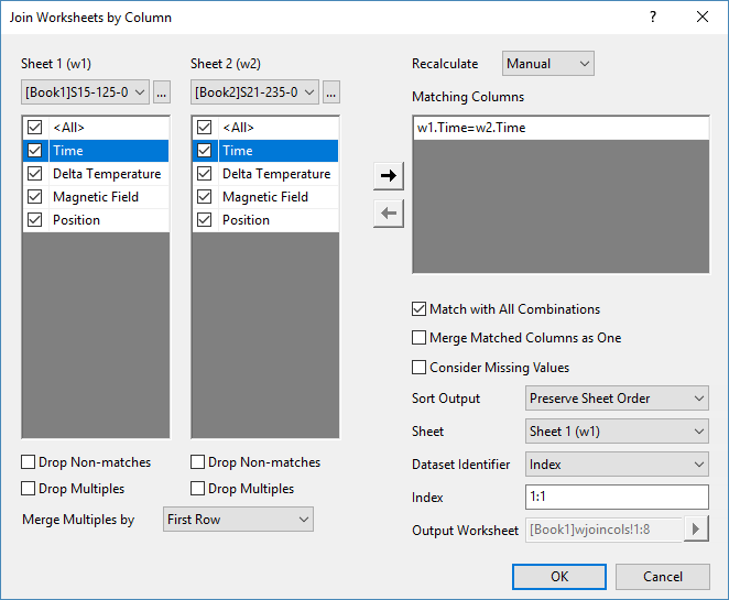
Specify the Recalculate Mode.
The left panel of the dialog has two column tables, w1 and w2. Checkboxes under each table control the settings of its owned sheet, respectively.
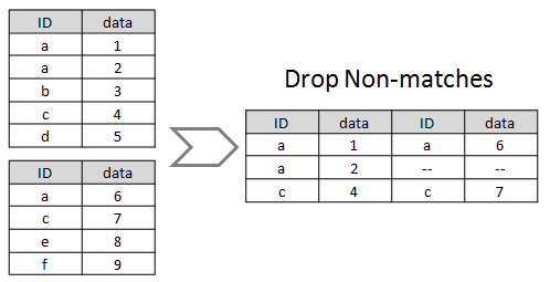
To exclude the unmatched cells from the joined worksheet, check this checkbox. Otherwise, columns of non-match values will fill with missing values.
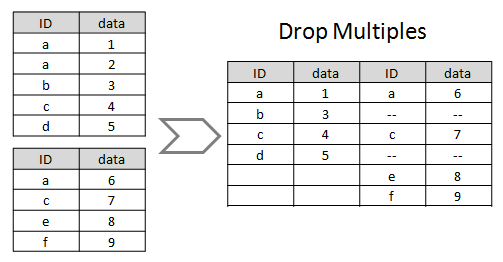
This is supposed to be used when there are multiple matched cells for one value. Check this checkbox to merge the multiples by statistics value specified in Merge Multiples by and the replica will be dropped.
Check the matching columns in w1 and w2 column table and click -> button to add the condition of joining worksheets in Matching Columns table. If multiple conditions exist, all conditions must be matched.
For example, if w1.A=w2.A is specified in Matching Columns, all values in column A of both sheet w1 and w2 will be compared and the matched rows will be combined as the same row in the joined worksheet..
Suppose all options are set to 0:
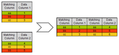
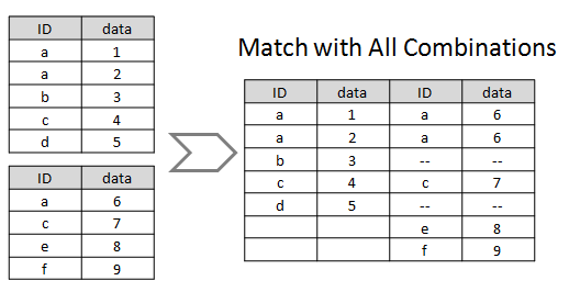
When there are multiple matched cells for one value, you can check this check box to show all possible combinations in result worksheet.
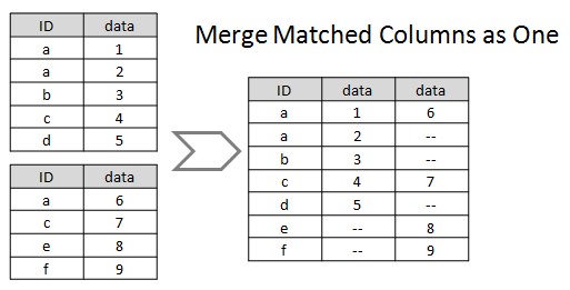
Specify whether to keep only one matching column in the joined worksheet.
Check this checkbox to consider missing value in the matching columns as a value to be compared. Uncheck will ignore rows with missing value.
Control how to sort the order of matched values in the joined sheet:
Specify whether to add a parameter label row named Source to the joined worksheet for identifying the source of dataset.
1:2 will identify columns from w1 as "1" and w2 as "3".