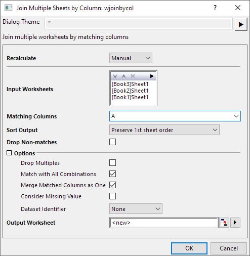
When you have multiple worksheets and want to combine them by column, considering that there are reference columns which should be matched, you can use the Join Multiple Sheets by Column tool.
To open this tool,
This tool utilizes the Wjoinbycol X-Function.
Specify the Recalculate Mode.
Specify the input worksheets you want to join. See the details about how to select input worksheets with the display box and toolbar.
[BookName1]SheetName1!ColumnShortName1=[BookName2]SheetName2!ColumnShortName2=[BookName3]SheetName3!ColumnShortName3
Control the order of matched values in the result sheet.
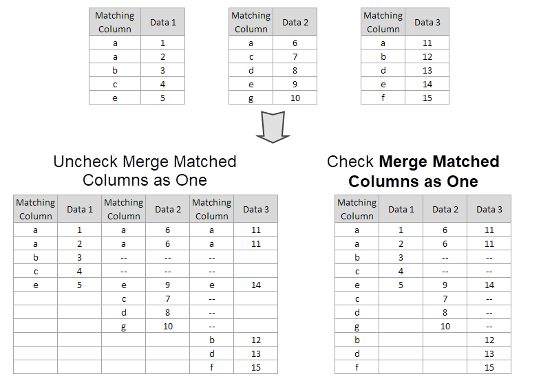
If Merge Matched Columns as One is not selected, Matching Columns – Ascending/Descending will sort output columns rather than matching columns by the first sheet order.
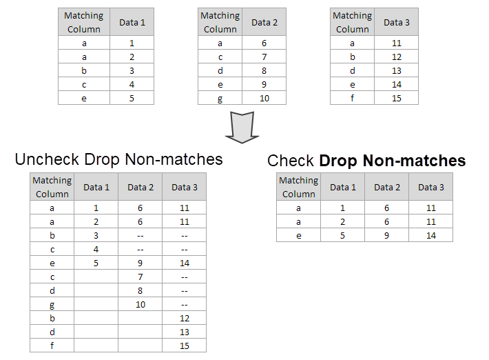
To exclude the unmatched cells from the joined worksheet, check this checkbox. Otherwise, columns of non-match values will fill with missing values.
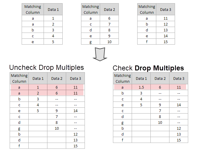
This is supposed to be used when there are multiple matched cells for one value. Check this checkbox to merge the multiples by statistics value specified in Merge Multiples by and the replica will be dropped.
Merge Multiples by: First, Last, Max, Min, Average & Sum.
When the Drop Non-matches option is checked, and set Merge Multiples by to Average, you get the result like this:
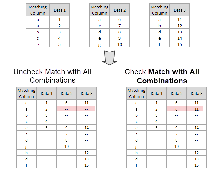
When there are multiple matched cells for one value, you can check this check box to show all possible combinations in result worksheet.
Specify whether to keep only one matched column in the result worksheet.
Check this checkbox to consider missing value in the matching columns as a value to be compared. Uncheck will ignore rows with missing value.
Specify whether to add a parameter label row named Source to the joined worksheet for identifying the source of dataset.
1:1 will identify source worksheets as 1,2,3,...| Note: When Merge Matched Column by On is checked, and Range/Book Name/Sheet Name/Index is selected as Identifier, Source label row of the matched column will show Merged. |
Specify the output worksheet.