From Origin 2019b, Notes window supports two modes: ordinary Edit Mode and Render Mode. When you edit a report according to HTML or Markdown syntax in Note Widows, you can show the report by render Mode. In the report, you can refer to Origin graph, image in matrix, analysis table and any worksheet cells. When the source changes, the linked in Notes window also get updated. This render mode makes it possible for Notes window to serve as an analysis report.
The default mode of Notes window is text mode. To switch to Render mode, you can use one of these four methods:
note.view=1;
| Notes: If you use Markdown syntax in the Notes Window, you must change Syntax to Markdown before changing to Render Mode. |
In Note widow, the edit mode default shows plain text as syntax option. When you edit by HTML or Markdown syntax, you can change the Syntax option. The HTML will shows the colored of the HTML syntax , while the Markdown syntax could help the Render Mode identify it is using Markdown syntax.
To switch to Syntax option, you can use these methods:
note.syntax=0; //switch to plain text
note.syntax=1; //switch to colored HTML syntax
note.syntax=2; //switch to Markdown
note.syntax=3; //switch to Origin Rich Text
When Notes Windows in edit mode, check menu Notes: Display line numbers to show the line numbers.
You can add graphs and worksheets, cell values, tables, matrices, strings and variables to the active Notes window by one of two methods:
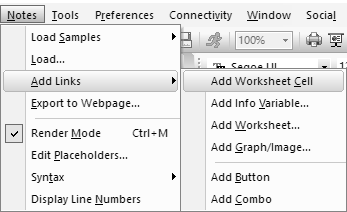
{{type://notation}}
Following link types are supported.
| type | notation | Description | Examples |
|---|---|---|---|
| graph | the graph window name | Insert a graph window as an image (.SVG). Note: If want to use .PNG style for the inserted image, set the system variable @NLS=0. | <img alt="{{graph://Graph1}}" width=400> |
| matrix | the matrix window name | Insert a matrix image. Note that you can Drag-n-Drop an image (jpg/png/bmp etc.) to a Notes window to insert it. The corresponding Matrix window is created and the syntax is auto-inserted into the Notes. | <img alt="{{matrix://matrix1}}"> |
| cell | range of the cell | Insert a worksheet cell content as a string. The syntax is [book_name]sheet_name!column_name[row-index]. |
{{cell://[book1]1!B[3]}} |
| table | range of the table | Insert a worksheet, table or cell (from report sheet) as a HTML table. The syntax is [book_name]sheet_name! or [book_name]sheet_name!table_name. |
{{table://[Book1]Sheet1!}}
|
| str | the Labtalk script of string | Insert string, for example Labtalk String Registers |
{{str://mystring$}}
|
| var | the Labtalk script of variable | Insert variable |
{{var://system.path.program$}} (display the program folder path)
|
| file | the file path | Insert file |
{{file://%@JSamples\Image Processing and Analysis\bamboo.jpg}}
|
|
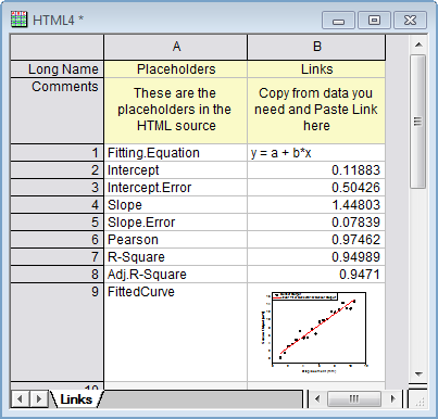
In the Notes window, it support use placeholders to insert link. These is a special Workbook named HTML to list the placeholders and the links.
To open the Workbook listed the placeholders:
In the Workbook, the first column are the name of the Placeholders, and cells in the second column lists the content of the links. You can insert variable and graph in the cell, and use this syntax to insert placeholders into the Notes window:
{{Placeholder}}
To add the links in the placeholder worksheet:
or
To insert LaTeX equation:
This will insert following MathJax scripts to render LaTeX notation in Markdown and HTML syntax:
<script src="http://olab/resource/ProgramData/OriginLab/JS/MathJax/config.js" defer></script>
<script type="text/javascript" id="MathJax-script" src=
"http://olab/resource/ProgramData/OriginLab/JS/MathJax/tex-svg.js" defer></script>
To see examples of inserting LaTeX equations, please select menu Notes: Load Samples: LaTeX Equations.html(md).
You can refer some of our build samples by selecting Notes: Load Samples:... in the menu.
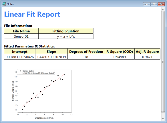
Here, we create a Linear Fit result report by HTML, HTML with Placeholders and Markdown respectively. You can compare their difference.
First, we need to prepare the analysis. Create a new project and import data <Origin installation folder>\Samples\Curve Fitting\Sensor01.dat into Book1. Change the window short name to be Sensor01. Highlight worksheet and create a scatter plot. Do a linear fit (Analysis: Fitting: Linear Fit) with default settings.
<html> <head> <style> td { text-align: center; } </style> </head> <body> <h1 style="color:#4285F4">Linear Fit Report</h1> <b>File Information:</b></br> <table class="origin-table centered" width="400px" > <tr> <th>File Name</th> <th>Fitting Equation</th> </tr> <tr> <td>Sensor01</td> <td>{{cell://[Sensor01]FitLinear1!Notes.Equation}}</td> </tr> </table> </br> <b>Fitted Parameters & Statistics:</b></br> <table class="origin-table centered" width="700px" > <tr> <th>Intercept</th> <th>Slope</th> <th>Degrees of Freedom</th> <th>R-Square (COD)</th> <th>Adj. R-Square</th> </tr> <tr> <td>{{cell://[Sensor01]FitLinear1!Parameters.Intercept.Value}}± {{cell://[Sensor01]FitLinear1!Parameters.Intercept.Error}}</td> <td>{{cell://[Sensor01]FitLinear1!Parameters.Slope.Value}} ± {{cell://[Sensor01]FitLinear1!Parameters.Slope.Error}}</td> <td>{{cell://[Sensor01]FitLinear1!RegStats.C1.DOF}}</td> <td>{{cell://[Sensor01]FitLinear1!RegStats.C1.RSqCOD}} </td> <td>{{cell://[Sensor01]FitLinear1!RegStats.C1.AdjRSq}}</td> </tr> </table> </br> <img alt="{{graph://Graph1}}" width=350> </body> </html>
<html> <head> <style> td { text-align: center; } </style> </head> <body> <h1 style="color:#4285F4">Linear Fit Report</h1> <b>File Information:</b></br> <table class="origin-table centered" width="400px" > <tr> <th>File Name</th> <th>Fitting Equation</th> </tr> <tr> <td>Sensor01</td> <td>{{Fitting.Equation}}</td> </tr> </table> </br> <b>Fitted Parameters & Statistics:</b></br> <table class="origin-table centered" width="700px" > <tr> <th>Intercept</th> <th>Slope</th> <th>Degrees of Freedom</th> <th>R-Square (COD)</th> <th>Adj. R-Square</th> </tr> <tr> <td>{{Intercept}}± {{Intercept.Error}}</td> <td>{{Slope}} ± {{Slope.Error}}</td> <td>{{DOF}} </td> <td>{{R-Square}} </td> <td>{{Adj.R-Square}}</td> </tr> </table> </br> <img alt="{{FittedCurve}}" width=350> </body> </html>
Compare the HTML syntax in Example1, you will find the placeholders help to simplify the HTML in Example2. |
# Linear Fit Report

**File Information:**
|File Name|Fitting Equation|
|--|--|
|{{File.Name}}|{{Fitting.Equation}}|


**Fitted Parameters & Statistics:**
|Intercept|Slope|Degrees of Freedom|R-Square (COD)|Adj. R-Square|
|--|--|--|--|--|
|{{Intercept}}±{{Intercept.Error}}|{{Slope}} ± {{Slope.Error}}|{{DOF}} |{{R-Square}}|{{Adj.R-Square}}

<img alt="{{FittedCurve}}" width=350>
Compare the HTML syntax in Example1, you will find Markdown syntax is easy to edit, but it can not support the some special styles in HTML. |