Univariate Spectral Density with Daniell Method
Tutorial
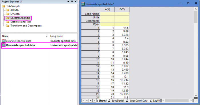
- Open the sample project file in Origin, go to Folder Spectral Analysis using the Project Explorer. Activate the workbook Univariate spectral data.
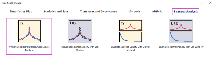
- Highlight column B in worksheet. Click the Time Series Analysis App icon
 in the Apps Gallery window.
- Choose Spectral Analysis tab. Click Univariate Spectral Density with Daniell Method icon to open the dialog.
- In the Setting branch, choose No correction. Enter 0.2,10 and 0.5 in Tapering Proportion, Smoothing Window Width and Shape Ratio of Trapezium Window respectively.
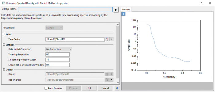
- Click Preview button to display smoothed spectrum.
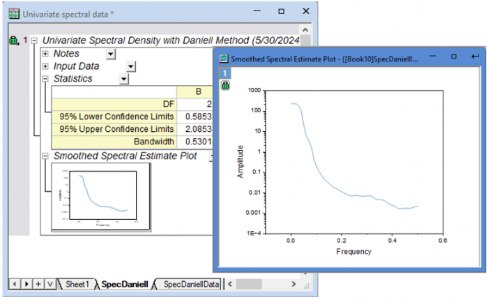
- Click OK button to output the report.
Algorithm
- \[\left\{\begin{array}{ll}\frac{1}{2}(1-cos(\frac{\pi(t-\frac{1}{2})}{T}))&1\leqslant t\leqslant T \cr\frac{1}{2}(1-cos(\frac{\pi(n-t+\frac{1}{2})}{T}))&n+1-T\leqslant t\leqslant n \cr1&Otherwise\end{array}\right.\]
- where \(T=[\frac{np}{2}]\) and \(p\) is the tapering proportion.
- The unsmoothed sample spectrum
- \[f^*(\omega) = \frac{1}{2}\pi|\sum_{t=1}^{n}x_texp(i\omega t)|^2\]
- is calculated for frequency values
- \[\omega_k = \frac{2\pi k}{K},k=0,1...,[K/2]\]
- where [ ] denotes the integer part.
- The smoothed spectrum is returned as a subset of these frequencies for which \(K\) is a multiple of a chosen value \(r\), i.e.,
- \[\omega_{rl}=v_l=\frac{2\pi l}{L},l=0,1,...,[L/2]\]
- where \(K=r\times L\)
Reference
- nag_tsa_spectrum_univar (g13cbc)