Tutorial for Decomposition
Notes for Starting
- Start this tutorial with the app Time Series Analysis installed. If you have not installed the app, see Apps for Origin to find and install the app.
Topics for Further Reading: |
User Story
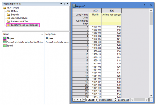
The dataset represents monthly international airline passenger totals (measured in thousands) for twelve consecutive years from 1960 to 1972. The dataset indicates a clear trend, because the airline industry enjoyed steady growth over the years. At the same time, the figures follow a seasonal pattern over 12 months.
An analysist wants to decompose the data and make forecasts for the next 6 months.
Steps in Origin
- Open the sample project file in Origin, go to Folder Transform and Decompose using the Project Explorer. Activate the workbook Airpass.
-
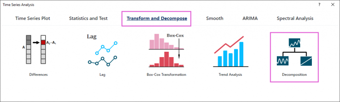
- Highlight column B in worksheet. Click the Time Series Analysis App icon
 in the Apps Gallery window.
 - Choose Transform and Decompose tab. Click Decomposition icon to open the dialog.
-
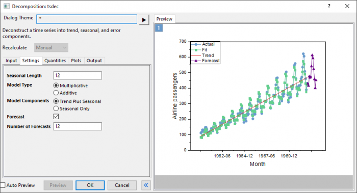
- In the Setting tab,set Seasonal Length to 12. Choose Multiplicative model type and Trend Plus Seasonal model components. Enter 12 in Number of Forecasts box.
-
- Click Preview button to display fitted curve with forecasts against actual data.
- Accept all other default settings and click OK button
Interpreting the Results
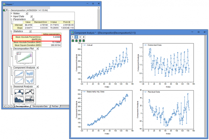
- The The mean absolute percent error (MAPE) value is 5.44%, indicating the fit data is 5.44% off the original data.It shows the model fits the data quite well.
- The Component Analysis plot include 4 graphs:
- Actual: Original data.
- Detrended Data: Data with the trend component removed from original data.
- Seasonally Adjusted Data: Data with the seasonal component removed from original data.
- Residuals: Difference between actual and fits.
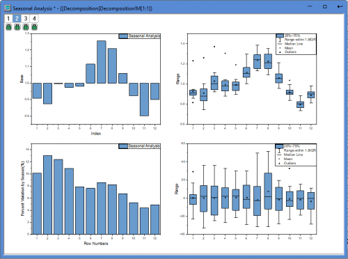
- The Seasonal Analysis plot include 4 graphs:
- Seasonal component plot (base = 1 for multiplicative model):It shows that the seasonal effect goes upward and reaches its largest in July (7th month), and then goes downward and reaches its smallest in November (11th month).
- Box chart for detrended data by season:Detrended data in November is most concentrated.
- Percent variation of detrended data by season:February has the largest variation and November has the smallest variation.
- Box chart for residuals by season:It does not show any obvious effect.