4.1.7 Quick Fit Gadget

Quick-Fit-Gadget

Quick Fit Gadget

Summary

The Quick Fit gadget can be used to quickly perform curve fitting within the ROI (Region of Interest) range.

Minimum Origin Version Required: Origin 8.6 SR0

What you will learn

This tutorial will show you how to:

• carry out linear fit with the Quick Fit gadget.
• carry out nonlinear curve fit using Quick Fit gadget.
• save and reuse a dialog theme.

Steps

Linear Fit

1. Open Origin and choose Data: Import from File: Import Wizard. For the Data Source, browse to <Origin Folder>/Samples/Curve Fitting and add the Step01.dat. Note that when this file is selected, the import filter Data Folder: step is automatically chosen (this is shown in in the Import Filters for Current Data Type box). Click Finish to import the file.
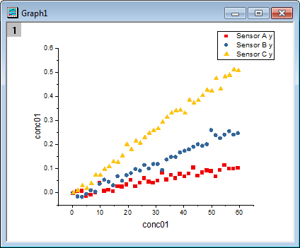
2. Highlight through column A to F and click the button to generate a scatter plot.

   

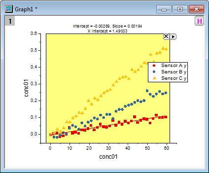
3. Select Gadgets: Quick Fit: 1 Linear(System) from the main menu to add a region-of-interest (ROI) box on the graph. Click the arrow button and select Expand to Full Plot(s) Range from the fly-out menu to expand the ROI box to the full plot range.

   

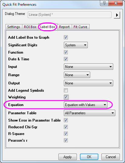
4. Click the arrow button and select Preferences... from the fly-out menu. This opens the Quick Fit Preferences dialog. In this dialog, go to the Label Box tab, select Equation with Values for the Equation drop-down list.

   

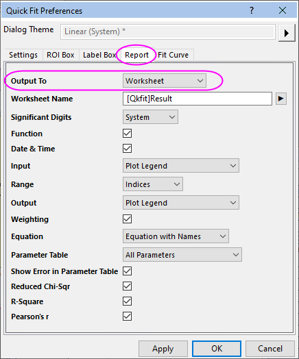
5. Go to the Report tab, select Worksheet for the Output To drop-down list.

   

6. Click OK to close this dialog. Click the arrow button to select New Output from the fly-out menu. This outputs the plot fitting results "Sensor 01" to the report worksheet and adds a label box to the graph window. The label box reports your analysis results.

   

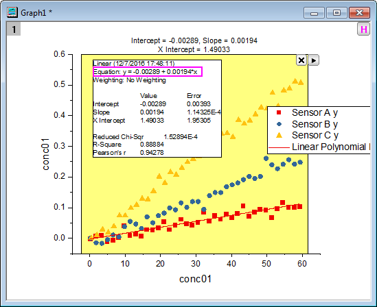
7. Select the label box on the graph and delete it. Click the arrow button and select Preferences... from the fly-out menu. This opens the Quick Fit Preferences dialog. In this dialog, go to Label Box tab, uncheck the Add Label Box to Graph check box and click OK.
8. Click the arrow button again to select New Output for All Curves(N) from the fly-out menu, so that the customized linear fit process will be performed on all data plots.
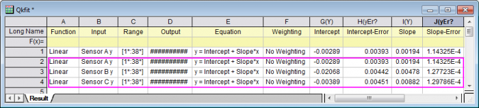
9. Click the arrow button one more time to select Go to Report Worksheet. You will see the fitting results of all three plots in the report worksheet. Note, the first result row has been created at step 6 above and the last three rows are our current results.

   

Note: With the ROI box shown on graph, you can click the arrow button to select Switch to Linear Fit... from the fly-out menu to transfer your current settings to the Linear Fit dialog. Then, you can do further operations in this more powerful dialog to do linear fitting.

Nonlinear Curve Fit

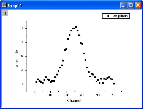
1. Start with a new workbook and import the Origin sample data Gaussian.DAT which is located in <Origin Program Folder>\Samples\Curve fitting path.
2. Highlight the Col(B) and select Plot>2D: Scatter: Scatter from the Origin menu to draw a graph.

   

3. Select Gadgets: Quick Fit: 4 Peak - Gauss (System) from the Origin menu to add a ROI box to the graph.

   

4. Click the arrow button to select Expand to Full Plot(s) Range from the fly-out menu to expand the ROI box to the full plot range.
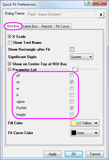
5. Click the arrow button and select Preferences... from the fly-out menu. This opens the Quick Fit Preferences dialog. In this dialog, go to the ROI Box tab, and set the Parameter List as below.

   

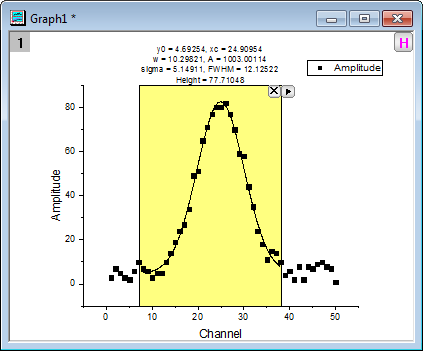
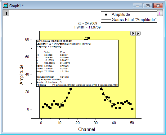
6. Click OK to close this dialog. Click the arrow button and select New Output from the fly-out menu. A label box will be added to the graph as shown below.

   

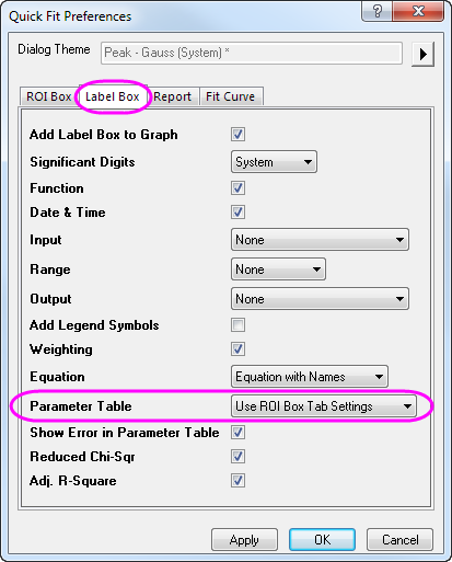
7. Click the arrow button and select Preferences... from the fly-out menu. This opens the Quick Fit Preferences dialog again. In this dialog, go to the Label Box tab, choose Use ROI Box Tab Settings for Parameter Table. Click OK to close this dialog.

   

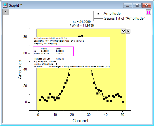
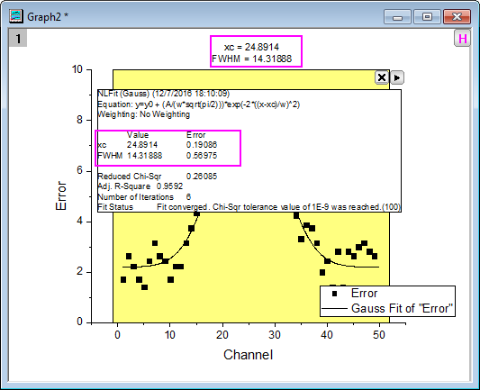
8. Click the arrow button and select Update Last Output from the fly-out menu. The Label box will be updated and only the parameters "xc" and "FWHM" will be displayed.

   

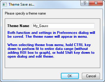
9. Click the arrow button and select Save Theme from the fly-out menu. In the Theme Save as... dialog, set the Theme Name as My_Gauss and click OK.

   

10. Go back to the worksheet, highlight col(C) and select Plot>2D: Scatter: Scatter from the top menu. This draws a scatter graph.
11. Click on the new plot to activate it and select Gadgets: Quick Fit: 9 My_Gauss to load the theme. A ROI box will be added to the graph with parameters xc and FWHM displaying above the ROI.
12. Click the arrow button to select Expand to Full Plot(s) Range from the fly-out menu to expand the ROI box to the full plot range, and then select New Output from the fly-out menu to output the result. You can see that our theme is applied as the label box on the graph only reports the values of parameter "xc" and "FWHM".

    

Note: With the ROI box shown on graph, you can click the arrow button to select Switch to NLFit... from the fly-out menu to transfer your current settings to the NLFit dialog. Then, you can do further operations in this more powerful dialog to do nonlinear fitting.