5.9 Power and Sample Size

Summary

Power and sample size analysis is useful in design of experiments. Insufficient data translates into a lack of power to reject a false null hypothesis and collecting too much data is a waste of time and resources. Therefore, it is essential to determine the sample size requirements prior to conducting an experiment. The power of the experiment can be computed for a given sample size, and required sample sizes can be computed for given power values.

What you will learn

This tutorial will show you how to calculate sample size or estimate power value to design experiments, using some practical examples.

(PSS)One-Sample t-Test

Background:
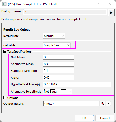
A sociologist wants to determine whether the average infant mortality rate in the United States is equal to 8. In experiment design, the difference of rate cannot vary more than 0.5. And it is already known that the standard deviation should be 2.1 from pilot studies.

Question:
What would the sample size be, in order to estimate the average infant mortality rate at a confidence level of 95% (\(\alpha\)=0.05) for power values of 0.7, 0.8 and 0.9?
Steps in Origin:

1. Activate an empty worksheet, select Statistics: Power and Sample Size: (PSS) One-sample t-test;
2. In the PSS_tTest1 dialog box, choose the following settings and click OK.

Origin Output:
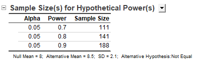
A result sheet will be generated, listing the calculated sample size for hypothetical powers.

Result Interpretation:
According to results, when designing his experiment the sociologist should conduct a survey of 111 samples for a power value of 0.7; 141 samples for power value of 0.8; and 188 samples for power value of 0.9.

(PSS)Two-Sample t-Test

Background:
A doctor's office participates in two local insurance plans, Healthwise and Medcare. The purpose is to compare the mean time (in days) until reimbursement of claims for the two plans. Historical data shows that for the Healthwise plan, the average time is 32 days and the standard deviation is 7.5 days. For the Medcare plan, the average reimbursement time is 42 days and the standard deviation is 3.5 days.

Question:
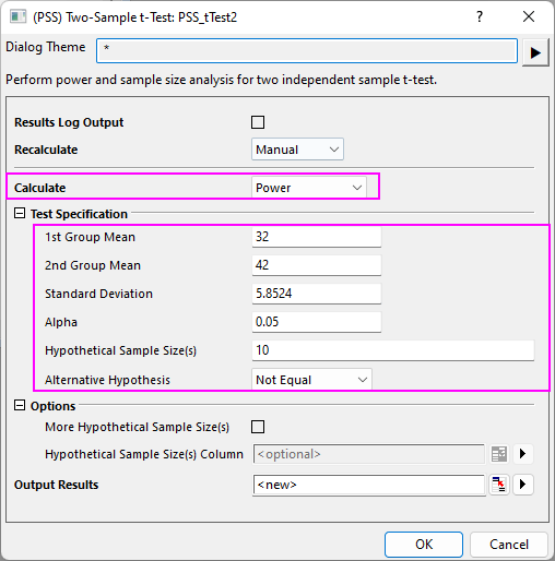
If 10 claims from each plan were selected and the corresponding reimbursement times were recorded, what is the power to detect the difference in mean reimbursement times between the 2 plans by 5% or more?

Steps in Origin:

1. Compute the pooled standard deviation as:

   \(\sqrt{((5-1)^{*}7.5^{\land} 2+(5-1)^{*}3.5^{\land }2)/(5+5-2)}=5.85235\)
   
   *Note that this value will be used as the standard deviation later for the power calculation.

2. Sample size of 1st group and 2nd group should be 10 (20 samples total).
3. Activate an empty worksheet and select Statistics: Power and Sample Size: (PSS) Two-Sample t-Test,
4. In the PSS_tTest2 dialog box, choose the following settings and click OK.
   

Origin Output:
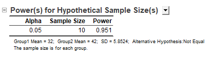
A result sheet will be generated, showing the calculated power.

Interpretation of Results:
We can conclude that the doctor's office has a 0.95054:1 (or 95%) chance of detecting a difference if it collects 10 claims for each plan. The chance that you will fail to reject the null hypothesis and incorrectly conclude that the two means are not different is 4.946% (1 - 0.95054).

(PSS)Paired-Sample t-Test

Background:
Two machines of the same type are used to measure the depth of an amorphous silicon (a-Si) thin film. To determine if there is a difference in the two machines measurements, an engineer plans a study to compare the depth measurements made by the two machines.

In a previous study on depth of the a-Si thin film, the standard deviation of the difference was found to be 2µm. In addition, it is known that the difference in measurement by the two machines should not exceed 0.5µm, and the average depth measured by Machine #1 is 5000µm.

Question:
How many samples must be taken at a confidence level of 99% to obtain power values of 0.8, 0.9 and 0.95?

Steps in Origin:
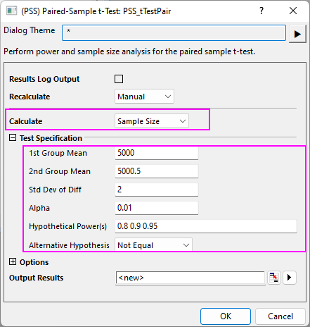
From the information above, it is concluded that the mean of the 1st group is 5000 µm and the mean of the 2nd group is 5000.5 µm.

1. Activate an empty worksheet and select Statistics: Power and Sample Size: (PSS) Paired t-Test
2. In the PSS_tTestPair dialog box, set controls as in the following image and click OK.

Origin Output:
A result sheet will be generated, listing the required sample size at different power values.

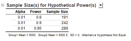
Interpretation of Results:
We conclude that the engineer has an 80% chance of detecting a difference if 191 thin film samples are measured; a 90% chance if 242 thin film samples are measured; and a 95% chance if 289 thin film samples are measured by each machine.

(PSS)One-Way ANOVA

Background:
Researchers are interested in whether different plants have different nitrogen contents. They planned to record nitrogen contents in milligrams for 4 species of plants (80 observations per species). Previous research suggests that the square root of MSE (Mean Squared Error) is 60 and the CSS (corrected sum of squares) of the means is 400.

Question:
Is the plan feasible? (i.e. will the calculated power be acceptable?)

Steps in Origin:

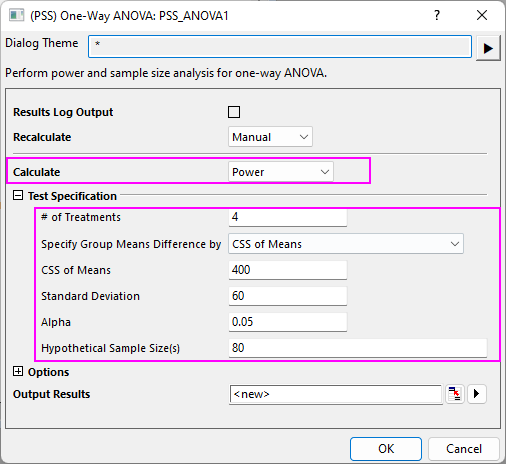
1. The sample size for each group is 80.
2. Activate an empty worksheet and select Statistics: Power and Sample Size: (PSS)One Way ANOVA
3. In the PSS_ANOVA1 dialog box, choose the following settings and click OK.

Origin Output:
A result sheet is generated, and the power value is calculated from the known condition.

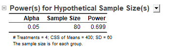
Interpretation of Results:
It appears that the original research plan is deficient. There is only a 69% chance of detecting a difference from each group. To get more reliable results, researchers must collect more samples per species of plant.

(PSS)One-Variance Test

Background:
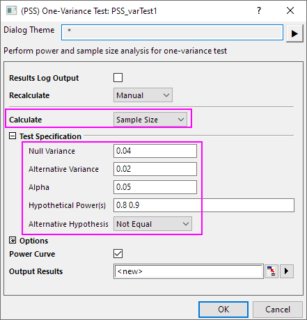
A semiconductor plant produces microchip packaging substrates. The Variance of the substrate thickness is a key indicator of process stability. Historical data (baseline) shows that the variance of the old process is 0.04. The engineering department has developed a new cooling system and claims it can reduce the variance to 0.02.

Question:
How many substrate samples does the quality control team need to test to detect this improvement with a Power of 0.8 and 0.9 (at a confidence level of \(\alpha\)=0.05 )?

Steps in Origin:

1. Go to the menu Statistics: Power and Sample Size: (PSS) One-Variance Test.
2. In the PSS_varTest1 dialog box, choose the following settings and click OK.
   

Origin Output:
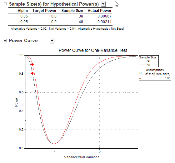
The results generated by Origin will show:

Interpretation of Results:

• To have an 80% chance of detecting a significant reduction in variance, at least 38 samples are required.

• To achieve a higher detection power of 90%, the sample size must be increased to 48.

(PSS)Two-Variance Test

Background:
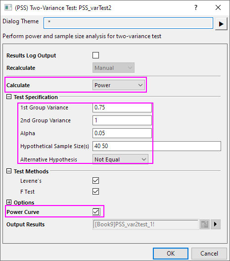
Researcher wants to evaluate the variability from two different groups. In preparation for the study, researcher collect 40, 50 samples from each group and are able to detect a standard deviation ratio of 0.75.

Question:
Researcher wants to know what the power of the 2 variances test.

Steps in Origin:

1. Go to the menu Statistics: Power and Sample Size: (PSS) Two-Variance Test.
2. In the PSS_varTest2 dialog box, choose the following settings and click OK.
   

Origin Output:
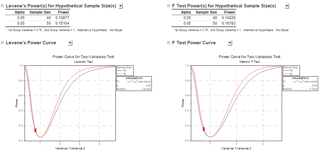
Levene's test and F test result

Interpretation of Results:

• From Levene's test, power is 0.12877 for sample size 40, and 0.15164 for sample size 50.

(PSS)One-Proportion Test

Background:
A precision component manufacturer maintains a strict quality standard where the defect rate must be kept below 2%. Recently, after switching to a new raw material supplier, the Quality Manager is concerned that the defect rate may have increased to 5%.

Question:
How many sample size is required to ensure sufficient statistical power to detect this shift?

Steps in Origin:

1. Go to the menu Statistics: Power and Sample Size: (PSS)One-Proportion Test.
2. In the PSS_proportionTest1 dialog box, choose the following settings and click OK.
   

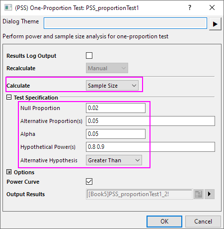
Note: We use a Greater Than test because the primary concern is the deterioration of quality (increase in defects).

Origin Output:
A result sheet will be generated, showing the calculated sample size.

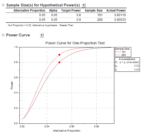
Interpretation of Results:
For a Power of 0.8, the required sample size is approximately 191. For a Power of 0.9, the required sample increases to approximately 289.

(PSS)Two-Proportion Test

Background:
It is known that a certain type of skin lesion will develop into cancer in 30% of patients if left untreated. There is a drug on the market that will reduce the probability of cancer developing by 10%. A pharmaceutical company is developing a new drug to treat skin lesions but it will only be worthwhile to do so if the new drug is 5% better than the existing drug. The pharmaceutical company plans to do a study with patients randomly assigned to two groups, the control (untreated) group and the treatment group.

Question:
The company wants to know how many subjects will be needed to test a difference in proportions of 0.15 with a power of 0.8 at alpha equal to 0.05.

Steps in Origin:

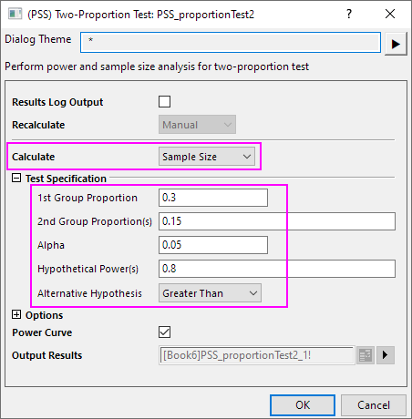
1. Go to the menu Statistics: Power and Sample Size: (PSS) Two-Proportion Test.
2. In the PSS_proportionTest2 dialog box, choose the following settings and click OK.
   

Origin Output:
A result sheet will be generated, showing the calculated sample size.

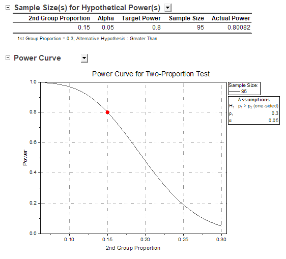
Interpretation of Results:
The results indicate that we need to use 95 subjects in each group to find a change in probability of 0.15 for a power of .8 when alpha equals 0.05.

(PSS)One-Sample Poisson Rate Test

Background:
A bank’s credit card customer service center has historical data showing that during the night shift (0:00 AM – 6:00 AM), the average number of emergency calls received is 5 per hour . Following a recent system upgrade, management is concerned that the frequency of these calls may have significantly increased. If the rate rises to 8 calls per hour, the current staffing level will be insufficient to handle the volume.

Question:
Calculate the required Length of Observation to ensure 80%/ 90%/ 95% power to detect a shift from 5 to 8 calls per hour.

Steps in Origin:

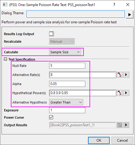
1. Go to the menu Statistics: Power and Sample Size: (PSS)One-Sample Poisson Rate Test.
2. In the PSS_poissonTest1 dialog box, choose the following settings and click OK.
   

Origin Output:

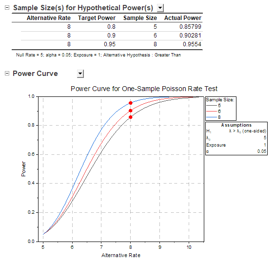
Interpretation of Results:
Origin will output a Sample Size is 5. That means it needs to monitor the call volume for a total of 5 hours. By observing for 5 hours, the total expected count shifts from 25 (5*5) to 40 (5*8), providing enough data to distinguish the increase from random fluctuations with 80% Power. To achieve higher power value, it requite to increase time length.

(PSS)Two-Sample Poisson Rate Test

Background:
A municipal transportation department is testing two types of asphalt (Material A and Material B). They aim to determine if Material B is safer than Material A by comparing the number of traffic accidents per unit distance. Historical data of Material A shows an accident rate of 12 per 10,000 km. The new Material B is expected to reduce the rate to 8 per 10,000 km

Question:
Determine the total distance (Sample Size) to be monitored for each material to achieve 80% Power.

Steps in Origin:

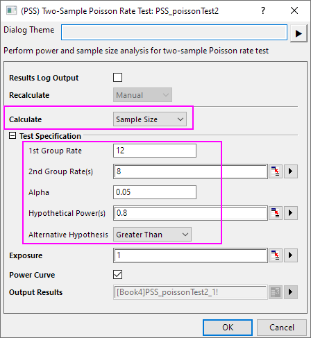
1. Go to the menu Statistics: Power and Sample Size: (PSS)Two-Sample Poisson Rate Test.
2. In the PSS_poissonTest2 dialog box, choose the following settings and click OK.
   

Origin Output:
A result sheet will be generated, showing the calculated sample size.

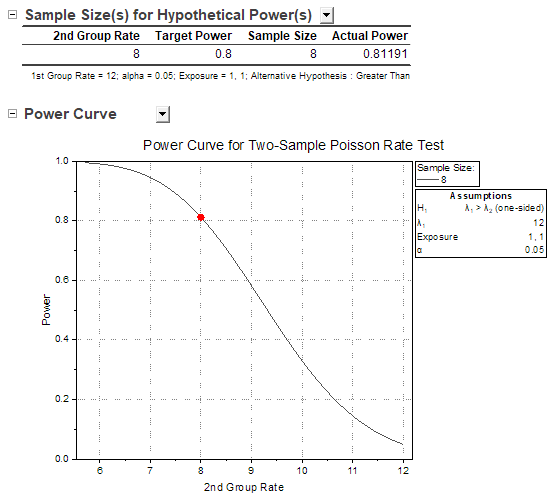
Interpretation of Results:
The calculation is a sample size of approximately 8 is required for each group. This implies the department must monitor 80,000 km of each pavement type to reliably detect the safety improvement.

Sample Size for Estimation

Background:
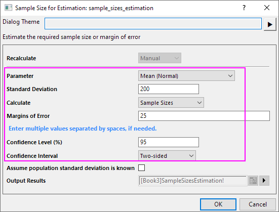
An component manufacturer has developed a new ceramic ball bearing. Before the product release, the R&D team must certify the "Mean Time to Failure" (MTTF) to be printed in the technical specifications. Accroding to the pilot study (a small-scale preliminary test), engineer calculate Standard Deviation about 200h from the 5 to 10 samples.

Question:
When the estimate hours must be within ±25 hours of the true mean, how many components need to be test to ensure the test result at 95% confidence interval?

Steps in Origin:

1. Go to the menu Statistics: Power and Sample Size: Sample Size for Estimation.
2. In the sample_size_estimation dialog box, choose the following settings and click OK.
   

Origin Output:
A result sheet will be generated, showing the calculated sample size.

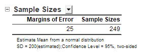
Interpretation of Results:
It need to test at least 249 individual components to ensure that your estimated mean is accurate within a Margin of Error of ±25 hours at a 95% Confidence Level.