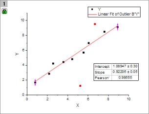
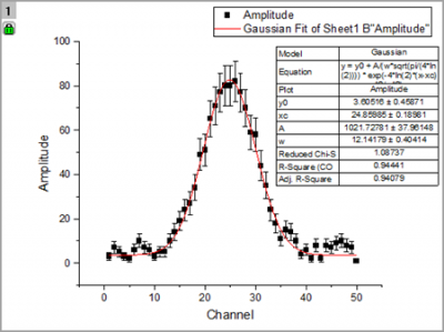
In this lesson we will learn how to perform linear and nonlinear regression.
Linear Fit with Outliers
Start with the project saved from the previous lesson, and add a new folder at the root level in Project Explorer named Curve Fitting.
Import the file <Origin EXE Path>\Samples\Curve Fitting\Outlier.dat by draging-and-droping the file into an empty worksheet.
Select the 2nd column and create a scatter plot.
Select the menu item Analysis: Fitting: Linear Fit. In the dialog that opens, accept default settings and click OK to perform the linear fit.
In the graph, click on the fitting results table and select Quantities in Table button from pop-up mini toolbar. Remove all entries except Intercept, Slope and Pearson's r (use CTRL + select for multiple selections). Click OK and resize the results table as needed.
Now click the Mask Points on Active Plot button on the left side toolbar and mask the point at the right bottom, which is distinctly separated from the rest of data points.
The lock on the top left of the graph page turns yellow indicating that the data has changed, but the fit results are in need of an update.
Hit the ESC key to switch the cursor back to pointer mode. Then click on the yellow lock, and from the fly-out menu select Recalculate Mode: Auto. The fit results will be updated.
You can update all pending operations in a project by clicking on the Recalculate button located in the Standard toolbar.
Go back to the graph and use the masking tool to mask the outlier point towards the top. You will notice that the results automatically update. Your graph should now look similar to this image:
Nonlinear Curve Fit
Start with a new workbook, and import the file <Origin EXE Path>\Samples\Curve Fitting\Gaussian.dat.
Highlight the column named Amplitude and make a scatter plot.
Go back to workbook, highlight column named Error, then select Set As Y Error button from pop-up mini toolbar.
Place the mouse cursor close to the right edge of the highlighted column. The cursor will change to . At this point, drag and drop the column onto the graph. The data will be added as error bars on the scatter plot.
Now let's fit this data. Select the menu Analysis: Fitting: Nonlinear Curve Fit to open then NLFit dialog.
In the Function Selection page, set Category drop down to Peak Functions, and set the Function drop down to Gauss.
Click Fit button to perform fitting and choose No in the prompt dialog, to keep the graph window active.
Now we want to fix y0 as 0 and update the results. Click on the green lock on the top left of the graph page, and select Change Parameters.
The dialog re-opens with the settings that were used last time the operation was performed. Go to the Parameters tab, check the Fixed box for y0 and enter Value as 0.
Click the Fit button to update the file and close the dialog. From the updated table on the graph, we can see that .
Global Fit with Parameter Sharing
Start a new workbook and import the file <Origin EXE Path>\Samples\Curve Fitting\Exponential Decay.dat.
Drag and select the three Y columns and create a line plot.
We want to fit all three data plots simultaneously over the x range of 0.4 s to 1.0 s. In the Tools toolbar docked to the left side of the interface, click the down arrow button on the right of Selection on Active Plot button . From the fly-out, choose Selection on All Plots. Go to the graph and drag and draw a rectangle to roughly cover the x range of 0.4 to 1.0, including all the three curves in the process.
Press CTRL+Y to quickly launch the NLFit dialog. Then set Category as Exponential and Function as ExpDec1.
Click on Data Selection under the Settings tab, expand the Input Data node and you will find all three curves are added. You can expand the Range# node to further adjust data ranges either by row index or by x value.
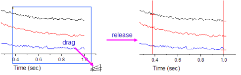
If no range selection has been made on the multiple plots, Origin will only pick up the active data plot from the graph layer containing multiple plots. In that case you can click the button on the right side of Input Data and select Add all plots in active page.
Change Multi-Data Fit Mode to Global Fit, switch to the Parameters tab and click the Fit until converged button to fit all three curves simultaneously, keeping the dialog open.
You can share parameters during a global fit. Check the Share box for the time constant t1. You will notice that the time parameter for the other curves has been removed from the parameters list.
Click the Fit button and select Yes in the prompt that appears, to switch to report sheet. If the prompt does not come up, you can click on the green lock in the graph and select Go to Results.
Scroll down to the Summary table in the report. You will find that all time constants t1 share the same values.
Now click on the down arrow button beside the Summary node and choose Create Copy as New Sheet. A new worksheet with the fit results will be added to the book.
Select column D, E and create a column plot to display how the amplitude parameter (A1) changed across the three datasets.