4.2.2.24 Fitting Integral Function with a Sharp Peak

Fitting-Integral-SharpPeak

Summary

In this tutorial, we will show you how to define an integral fitting function with a sharp peak in the integral function, and perform a fit of the data using this fitting function.

Because the integral function contains a sharp peak, the integral should be performed in three segments so that the sharp peak can be integrated in a narrow interval.

Minimum Origin Version Required: Origin 9.0 SR0

What you will learn

This tutorial will show you how to:

• Define an integral fitting function.
• Integrate a function with a sharp peak.
• Divide the integral interval into several segments.

Example and Steps

Import Data

1. Open a new workbook.
2. Copy data in Sample Data to the workbook.
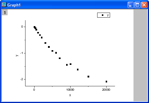
3. Highlight column B, and select Plot: Symbol: Scatter from Origin menu. The graph should look like:

Define Fitting Function

The fitting integral function is described as follows:

where a and b are parameters in the fitting function.

Initial parameters are: a=1e-4, b=1e-4. Note that the integral function contains a peak whose center is about a and width is 2b. And the peak's width (2e-4) is very narrow compared with the integral interval [0,1]. To make sure it is integrated correctly at the neighborhood of the peak center, the integral interval [0,1] is divided into three segments: [0,a-5*b], [a-5*b,a+5*b], [a+5*b,1]. It is integrated in each segment, and then the three integrals are summed up.

The fitting function can be defined using the Fitting Function Builder tool.

1. Select Tools: Fitting Function Builder from Origin menu.
2. In the Fitting Function Builder dialog's Goal page, click Next button.
3. In the Name and Type page, select User Defined from Select or create a Category drop-down list, type fintpeak in the Function Name field, and select Expression in Function Type group, check Include Integration During Fitting check box. And click Next button.
4. In the Integrand page, type myint in Integrand Name edit box, t in Integration Variable edit box and a, b, x in Arguments edit box. Type the following script in Integrand Function box.

   return 1/(sqrt(2*pi)*b)*exp(-(t-a)^2/(2*b^2)-x*t);

   And click Next button.

5. In the Variables and Parameters page, type a, b in the Parameters field. Click Next button.
6. In the Expression Function page, click Parameters tab, and set Initial Value for parameters a and b to 1e-4, click Integrand tab, and set Value for Lower Limit and Upper Limit to 0 and 1, Value for a, b, x to a, b, x respectively.
7. In the Expression Function page, click Insert button. In the Quick Check group, type 0 in x= edit box, click Evaluate button, and it shows y=9.3e-21. This implies that the peak is not integrated correctly because y should approach 1 for x=0. Divide the integral into three segments, and type following script in Function Body box.

   integral(myint, 0, a-5*b, a ,b ,x)+integral(myint, a-5*b, a+5*b, a ,b ,x)+
   integral(myint, a+5*b, 1, a ,b ,x)

   Click Evaluate button again, and it shows y=0.84, hence it is clear that the peak is integrated correctly this time.

8. In the Expression Function page, update the script in Function Body box as follows.

   log(integral(myint, 0, a-5*b, a ,b ,x)+integral(myint, a-5*b, a+5*b, a ,b ,x)
   +integral(myint, a+5*b, 1, a ,b ,x))

   Click Finish button.

Fit the Curve

1. Select Analysis: Fitting: Nonlinear Curve Fit from Origin menu. In the NLFit dialog, select Settings: Function Selection, in the page select User Defined from the Category drop-down list and fintpeak function from the Function drop-down list. Note that initial parameters have been set during defining the fitting function.
2. Click Fit button to fit the curve.

Fitting Results

The fitted curve should look like:

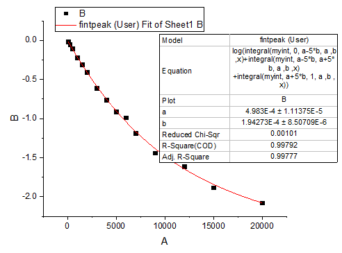
Fitted Parameters are shown as follows:

Parameter	Value	Standard Error
a	4.98302E-4	1.07593E-5
b	1.94275E-4	8.21815E-6

The Adj. R-Square is 0.99799. Thus the fitting result is very good.

Sample Data

x	y
0	-0.00267
60	-0.01561
240	-0.05268
500	-0.10462
1000	-0.22092
1500	-0.31004
2000	-0.40695
3000	-0.61328
4000	-0.75884
5000	-0.9127
6000	-0.98605
7000	-1.18957
9000	-1.43831
10000	-1.41393
12000	-1.61458
15000	-1.88098
20000	-2.07792