If your data is a convolution of Gauss and Exponential functions, you can simply use built-in fitting function GaussMod in Peak Functions category to directly fit your data.
When performing curve fitting to experimental data, one may encounter the need to account for instrument response in the data. One way to do this is to first perform deconvolution on the data to remove the instrument response, and then perform curve fitting as a second step. However, deconvolution is not always reliable as the results can be very sensitive to any noise present in the data. A more reliable way is to perform convolution of the fitting function with the instrument response while performing the fitting. This tutorial will demonstrate how to perform convolution while fitting.
If your data is a convolution of Gauss and Exponential functions, you can simply use built-in fitting function GaussMod in Peak Functions category to directly fit your data. |
Minimum Origin Version Required: Origin 2016 SR0.
This tutorial will show you how to:
Let's start this example by importing \Samples\Curve Fitting\FitConv.dat.
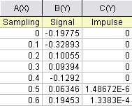
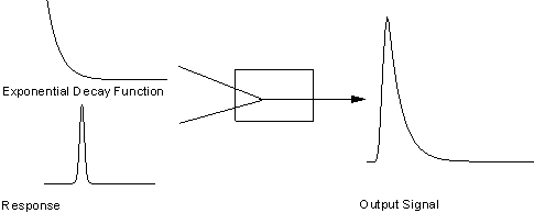
The source data includes sampling points, output signal, and the impulse response. This experiment assumes that the output signal was the convolution of an exponential decay function with a Gaussian response:
Now that we already have the output signal and response data, we can get the exponential decay function by fitting the signal with the below model:

Obviously, column 1 and column 2 are x and y respectively in the function. How about column 3, the impulse response? We will access this column within the fitting function, and compute the theoretical exponential curve from the sampling points. Then we can use fast Fourier transform to perform the convolution.
Press F9 to open the Fitting Function Organizer and define a function like:
| Function Name: | FitConv |
| Function Type: | User-Defined |
| Independent Variables: | x |
| Dependent Variables: | y |
| Parameter Names: | y0, A, t |
| Function Form: | Origin C |
| Function: |
Click the button (icon) beside the Function box and write the function body in Code Builder:
#pragma warning(error : 15618)
#include <origin.h>
// Header files need to be included
#include <ONLSF.H>
#include <fft_utils.h>
//
//
void _nlsfFitConv(
// Fit Parameter(s):
double y0, double A, double t,
// Independent Variable(s):
double x,
// Dependent Variable(s):
double& y)
{
	// Beginning of editable part
	NLFitContext *pCtxt = Project.GetNLFitContext();
        Worksheet wks;
        DataRange dr;
        int c1,c2;
        dr = pCtxt->GetSourceDataRange(); //Get the source data range
        dr.GetRange(wks, c1, c2);  //Get the source data worksheet
	if ( pCtxt )
	{
		// Vector for the output signal in each iteration.
		static vector vSignal;
		// If parameters were updated, we will recalculate the convolution result.
		BOOL bIsNewParamValues = pCtxt->IsNewParamValues();
		if ( bIsNewParamValues )
		{
			// Read sampling and response data from worksheet.
			Dataset dsSampling(wks, 0);
			Dataset dsResponse(wks, 2);
			int iSize = dsSampling.GetSize();

			vector vResponse, vSample;

			vResponse = dsResponse;
			vSample = dsSampling;

			vSignal.SetSize(iSize);
			vResponse.SetSize(iSize);
			vSample.SetSize(iSize);

			// Compute the exponential decay curve
			vSignal = A * exp( -t*vSample );
			// Perform convolution
			int iRet = fft_fft_convolution(iSize, vSignal, vResponse);
                        //Correct the convolution by multiplying the sampling interval
                        vSignal = (vSample[1]-vSample[0])*vSignal;


		}

		NLSFCURRINFO    stCurrInfo;
		pCtxt->GetFitCurrInfo(&stCurrInfo);
		// Get the data index for the iteration
		int nCurrentIndex = stCurrInfo.nCurrDataIndex;
		// Get the evaluated y value
		y = vSignal[nCurrentIndex] + y0;
		// For compile the function, since we haven't use x here.
		x;
	}
	// End of editable part
}
Traditionally, for a particular x, the function will return the corresponding y value. However, when convolution is involved, we need to perform the operation on the entire curve, not only for a particular data point. So, from Origin 8 SR2, we introduced the NLFitContext class to achieve some key information within the fitter. In each iteration, we use NLFitContext to monitor the fitted parameters; once they are updated, we will compute the convolution using the fast Fourier transform by the fft_fft_convolution method. The results are saved in the vSignal vector. Then for each x, we can get the evaluated y from vSignal with the current data index in NLSFCURRINFO.
In the fitting function body, we read the response data directly from the active worksheet. So, you should perform the fit from the worksheet.
If you use a fitting function similar to this tutorial, please note when you run NLFit in Origin, in NLFit dialog, choose X Data Type from Fitted Curves page as Same as Input Data.