Bivariate Spectral Density with Lag Window
Tutorial
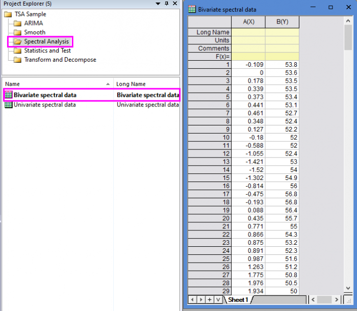
- Open the sample project file in Origin, go to Folder Spectral Analysis using the Project Explorer. Activate the workbook Bivariate spectral data.
-
- Highlight column A and B in worksheet. Click the Time Series Analysis App icon
 in the Apps Gallery window.
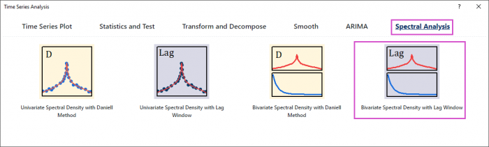
 - Choose Spectral Analysis tab. Click Bivariate Spectral Density with Lag Window icon to open the dialog.
-
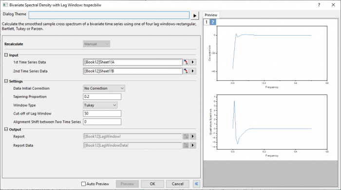
- In the Setting branch, choose No correction. Enter 0.2 in Tapering Proportion. Choose Tukey window type. Enter 50 and 0 in Cut-off of Lag Window and Aligment Shift between Two Time Series.
-
- Click Preview button to display smoothed spectrum.
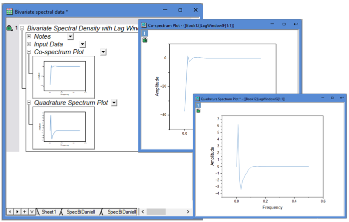
- Click OK button to output the report.
-
Algorithm
The smoothed sample cross spectrum is a complex valued function of frequency  ,
, =cf(\omega)+iqf(\omega)") , defined by its real part or co-spectrum
, defined by its real part or co-spectrum
=\frac{1}{2\pi}\sum_{k=-M+1}^{M-1}\omega_kC_{xy}(k+S)cos(\omega k)")
and imaginary part or quadrature spectrum:
=\frac{1}{2\pi}\sum_{k=-M+1}^{M-1}\omega_kC_{xy}(k+S)sin(\omega k)")
where  , for
, for  , is the smoothing lag window as described in Univariate Spectral Density with Lag Window.
The results are calculated for frequency values
![\omega_j = \frac{2\pi j}{L},j=0,1...,[L/2]](/tutorials/ja/images/Bivariate_Lag/math-a17d49c12718ff1f6716a9b6d001a028.png "\omega_j = \frac{2\pi j}{L},j=0,1...,[L/2]")
where [ ] denotes the integer part.
Reference