5.6.17 Bivariate Spectral Density with Daniell Method

Tutorial

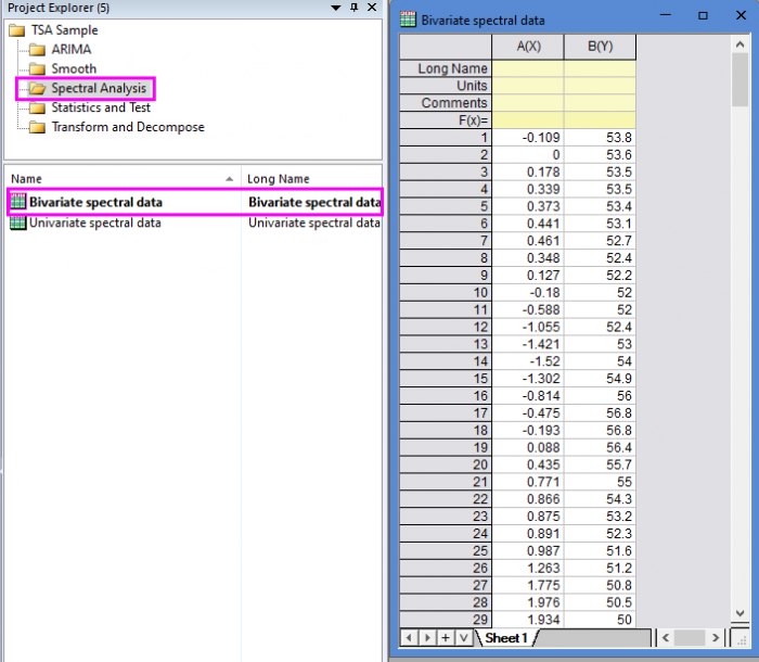
1. Open the sample project file in Origin, go to Folder Spectral Analysis using the Project Explorer. Activate the workbook Bivariate spectral data.

   

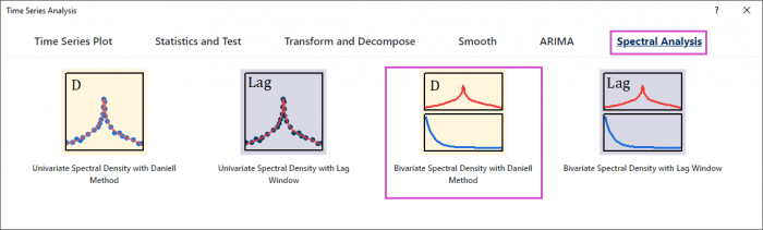
2. Highlight column A and B in worksheet. Click the Time Series Analysis App icon in the Apps Gallery window.
3. Choose Spectral Analysis tab. Click Bivariate Spectral Density with Daniell Method icon to open the dialog.

   

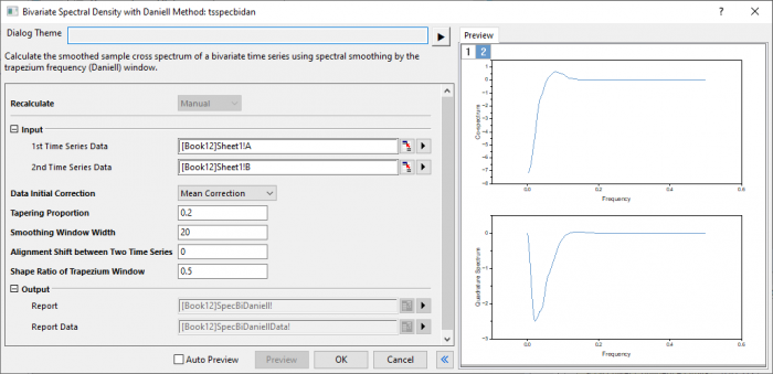
4. In the Setting branch, choose Mean correction. Enter 0.2,20, 0 and 0.5 in Tapering Proportion, Smoothing Window Width, Aligment Shift between Two Time Series, and Shape Ratio of Trapezium Window respectively.

   

5. Click Preview button to display smoothed spectrum.
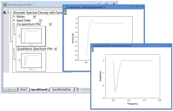
6. Click OK button to output the report.

   

Algorithm

• Smoothed sample cross-spectrum

The unsmoothed sample cross-spectrum

\[f^*_{xy}(\omega) = \frac{1}{2\pi n}(\sum_{t=1}^{n}y_texp(i\omega t))\times (\sum_{t=1}^{n}x_texp(-i\omega t))\]

for frequency values \(\omega_j = \frac{2\pi j}{K},0\le \omega_j \le \pi\).

The smoothed spectrum is returned at a subset of these frequencies

\[v_l=\frac{2\pi l}{L},l=0,1,...,[L/2]\]

where [ ] denotes the integer part.

Its real part or co-spectrum \(cf(v_l)\), and imaginary part or quadrature spectrum \(qf(v_l)\) are defined by

\[f_{xy}(v_l)=cf(v_l)+iqf(v_l)=\sum_{|\omega_k|<\pi/M}^{}\hat{\omega}_kf^*_{xy}(v_l+\omega_k)\]

where \(\hat{\omega}_k=\omega_kexp(-2\pi iSk/L)\), and \(S\) is alignment shift.

Reference

1. nag_tsa_spectrum_bivar (g13cdc)