4.4.22 Time Series Pivot

Origin supports Time Series Pivot tool to create a pivot table to visualize data summarization (of statistics) based on a date-time column

To open this tool, with a workbook window activated,

Select Restructure : Time Series Pivot... menu;

Run wtspivot -d; in Script Window or Command Window.

This tool utilizes the Wtspivot X-Function.

1 Recalculate
2 Source
3 Rows
4 Columns
5 Date/Time Window
6 Aggregate by
- 6.1 Custom
7 Show Zeros when Empty
8 Output
9 Samples

Recalculate

Specify the Recalculate Mode.

Source

Source Time	Select one column with date/time dataset
Source Data	Select the dataset(s) will be aggregated in the result sheet.

Rows

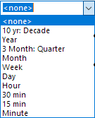
Aggregation Interval	Specify the aggregation interval of time in the rows of the pivot table. This time interval is shown in first column of the pivot table. You can select this options in this drop-down list：
Time Period	Specify the time group of the aggregation interval. According to the selected Aggregation Interval, you can select the corresponding time period. When 10yr:Decade is selected as Aggregation Interval, Time Period just can keep to <none>. When Year is selected as Aggregation Interval, you can select 10yr:Decade as Time Period. When 3 Month: Quarter, Month, Week or Day is selected as the Aggregation Interval, you can select Year as Time Period. When Week or Day is selected as Aggregation Interval, you can select Month as Time Period. When Day or Hour is selected as Aggregation Interval, you can select Week as Time Period. When 30 min, 15min or Minute is selected as Aggregation Interval, you need select Day or Hour as Time Period. The Time Period can not keep to <none>.
Remove Empty	Check this check box to remove the empty rows.
Start / End	Enter the start or end time of the rows of the pivot table. The time format of the Start and End is based on the selected Aggregation Interval. You can refer to the blue hint showing above this edit box. If keeps the edit box empty, the start or end time is default time of the table. Under the Rows setting, in the following situations, the Start / End box is hided. When Aggregation Interval=10yr:Decade When Aggregation Interval=3 Month: Quarter and Time Period=<none>
Custom Format	Custom the time format showing in the first column except some combinations of Aggregation Interval and Time Period. For example: when Aggregation Interval=Month and Time Period=Year, this the format can not be customized.

Columns

Aggregation Interval	Specify the aggregation interval of time in the columns of the pivot table. This time interval is shown in Comment label row of the pivot table. You can select this options in this drop-down list：
Time Period	Specify the time group of the aggregation interval. According to the selected Aggregation Interval, you can select the corresponding time period. When 10yr:Decade is selected as Aggregation Interval, Time Period just can keep to <none>. When Year is selected as Aggregation Interval, you can select 10yr:Decade as Time Period. When 3 Month: Quarter, Month, Week or Day is selected as the Aggregation Interval, you can select Year as Time Period. When Week or Day is selected as Aggregation Interval, you can select Month as Time Period. When Day or Hour is selected as Aggregation Interval, you can select Week as Time Period. When 30 min, 15min or Minute is selected as Aggregation Interval, you need select Day or Hour as Time Period. The Time Period can not keep to <none>.
Remove Empty	Check this check box to remove the empty columns.
Follow Rows Start	When the Start Value of Rows is bigger than End value and the Column’s Aggregation Interval is same as the Rows Time Period. The option is shown in the dialog. If the Row Time Period is set to Year or Week, etc. but it doesn’t start from the traditional start of the year or week, you can check this option to summarize data by Fiscal Year. If unchecked, all data of same calendar year/week will instead be put in one column.
Start / End	Enter the start or end time of the columns of the pivot table. The time format of the Start and End is based on the selected Aggregation Interval. You can refer to the blue hint showing above this edit box. If keeps the edit box empty, the start or end time is default time of the table. Under the Columns setting, in the following situations, the Start / End box is hided. When Aggregation Interval=10yr:Decade When Aggregation Interval=Year/3 Month: Quarter/Week/Day/Hour and Time Period=<none>
Custom Format	Custom the time format showing in the Comment label row except some combinations of Aggregation Interval and Time Period. For example: when Aggregation Interval=Month and Time Period=Year, this the format can not be customized.

Date/Time Window

Specify the date/time range to control the source date range that used to be aggregated.

Aggregate by

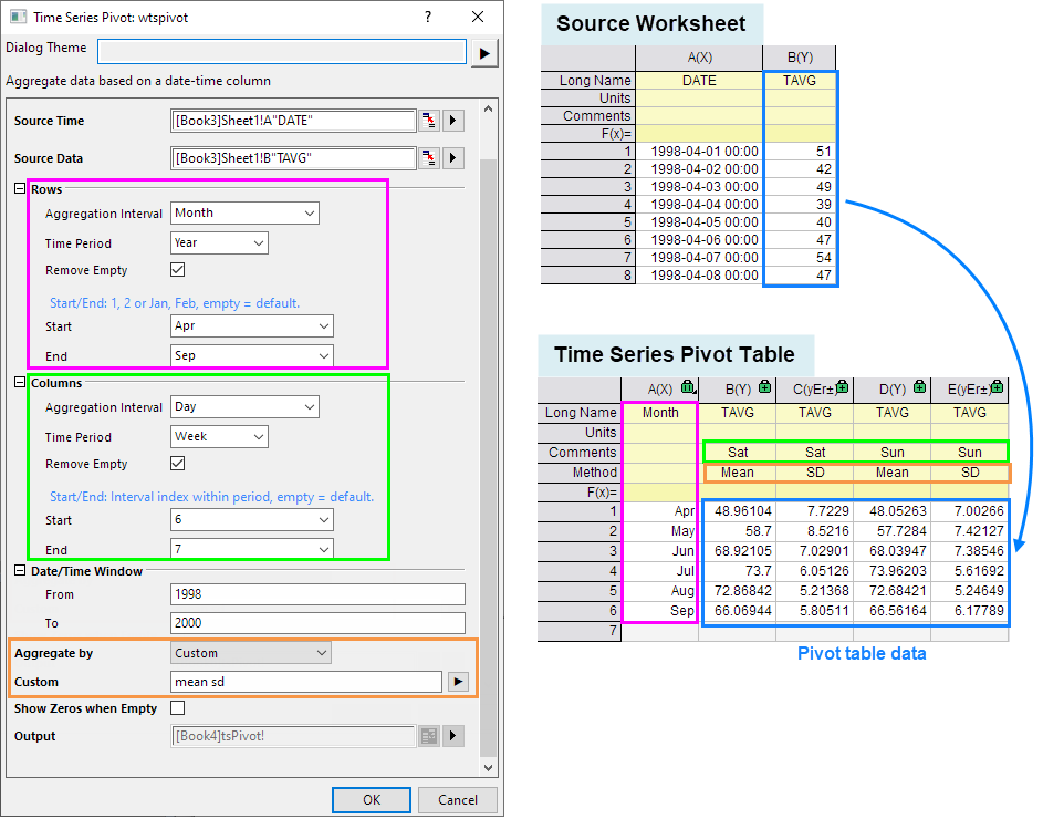
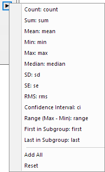
Select the aggregation method to summarize the Source Data, including

Custom

Available only when Aggregate by is set to Custom. Specify the summarized method in the combo edit box. The triangle button next to the edit box provides some frequently-used statistics quantities. You can mix them and construct your own summarized method. You also can add all methods or reset the selection by this menu.

Show Zeros when Empty

Specify whether to show missing values in the pivot table as zeros.

Output

Specify where to output the result time series pivot table tsPivot. Click the triangle button to specify output method.

[<input>]<input>: Input the time series pivot table into the current worksheet.

<new>: Put time series pivot table into a new sheet of the current workbook.

[<new>]<new>: Put time series pivot table into a new workbook.

Samples

Summarize Data Row-wise Only

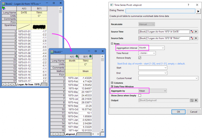
Here, We have a daily max temperature data from 1970-01-01 to 2023-12-31.

Sample1: To summarize the mean value of max temperature in each month during 1970 to 2023.

Set Aggregation Interval: Month in the Rows, then you can get the summarize data of max temperature in each month, and there is no Time Period, each month of different years will be a separate row.

Set Aggregation Interval: Month and Time Period: Year in the Rows, then the same month of different years will be summarized together so only 12 rows in output.

Summarize Data Both Column and Row-wise

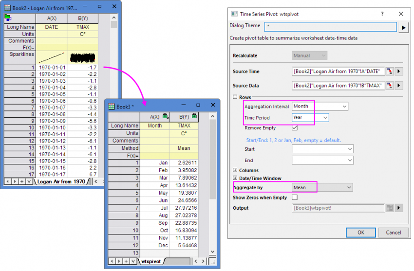
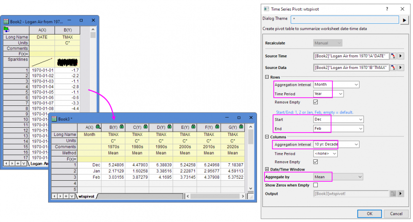
We go on using a daily max temperature data from 1970-01-01 to 2023-12-31.

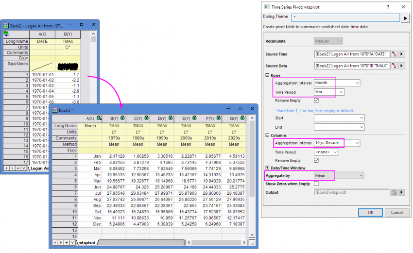
Sample2: To summarize the mean value of max temperature of each month for each decade.

Set Aggregation Interval: Month and Time Period: Year in the Rows, and Aggregation Interval: 10yr:Decade in the Columns.

If you just want to focus on the temperature changing in Winter, following above setting, and then set Start: Dec and End: Feb in the Rows.

Summarize Data by Fiscal Year

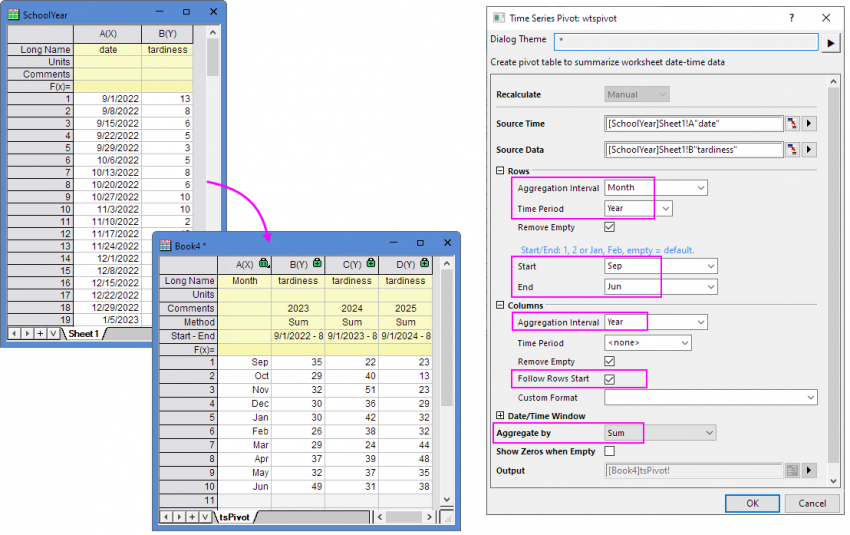
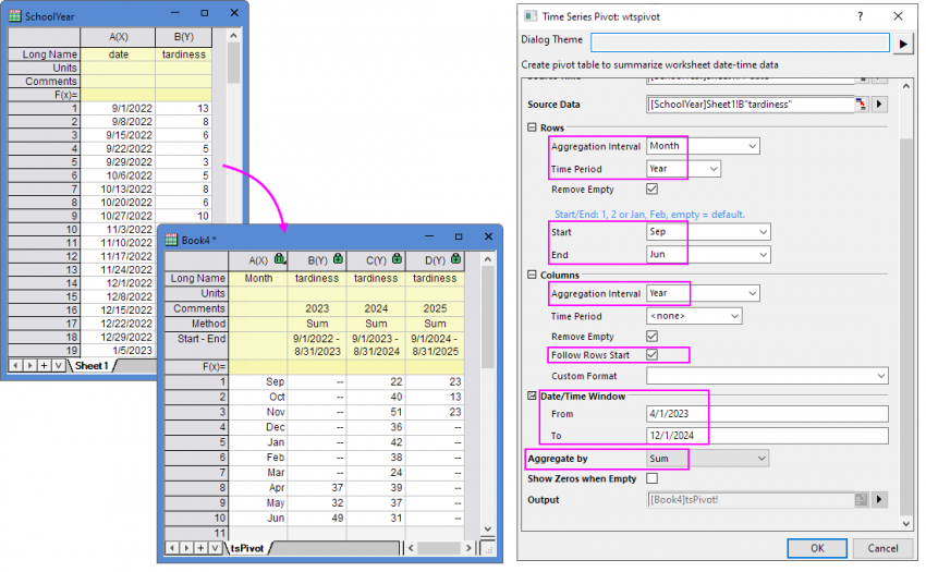
When the summarized data doesn’t start from the traditional start of the year or week, and the Row Time Period is set to Year or Week, etc, you can use Follow Rows Start to summarize data for Fiscal Year.

Here, we use a sample data of the tardiness of School Year from 9/1/2022 to 6/25/2025. This fiscal year starts from Sep. 1st and ends on Jun. 30th next year

Sample3: To summarize the sum value of the tardiness in each month for Fiscal Year.

Set Aggregation Interval: Month and Time Period: Year in the Rows, Aggregation Interval: Year in the Columns and check Follow Rows Start option.

If you want to specify the data range for the dataset, following above setting, and then fill the date/time range under Date/Time Window, for example from 4/1/2023 to 12/1/2024.