17.2.4 Probability Plot and Q-Q Plot

The probability plot is used to test whether a dataset follows a given distribution. It shows a graph with an observed cumulative percentage on the X axis and an expected cumulative percentage on the Y axis. If all the scatter points are close to the reference line, we can say that the dataset follows the given distribution.

A Q-Q (Quantile-Quantile) plot is another graphic method for testing whether a dataset follows a given distribution. It differs from the probability plot in that it shows observed and expected values instead of percentages on the X and Y axes. If all the scatter points are close to the reference line, we can say that the dataset follows the given distribution.

Origin supports five given distributions (Normal, Lognormal, Exponential, Weibull and Gamma), and five methods for plotting percentile approximations (Blom, Benard, Hazen, Van der Waerden, and Kaplan-Meier).

Creating Probability Plot or Q-Q Plot

To create a probability plot or Q-Q plot:

Highlight one Y column or multiple Y columns as input variable(s).
Open the probability/Q-Q plot dialog:
For a probability plot: In Origin's main menu, click Plot > Statistical: Probability Plot.... Alternatively, you can click the Probability Plot button on the 2D Graphs toolbar.

For a Q-Q plot: In Origin's main menu, click 'Plot > Statistical: Q-Q Plot.... Alternatively, you can click the Q-Q Plot button on the 2D Graphs toolbar.
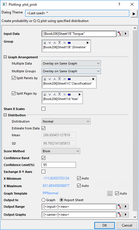
In the plot_prob X-Function dialog, select the grouping column(s), set arrangement of groups and variables, choose a column to split the plot into panels, specify the distribution and method.
Click OK to create a probability plot or a Q-Q plot.

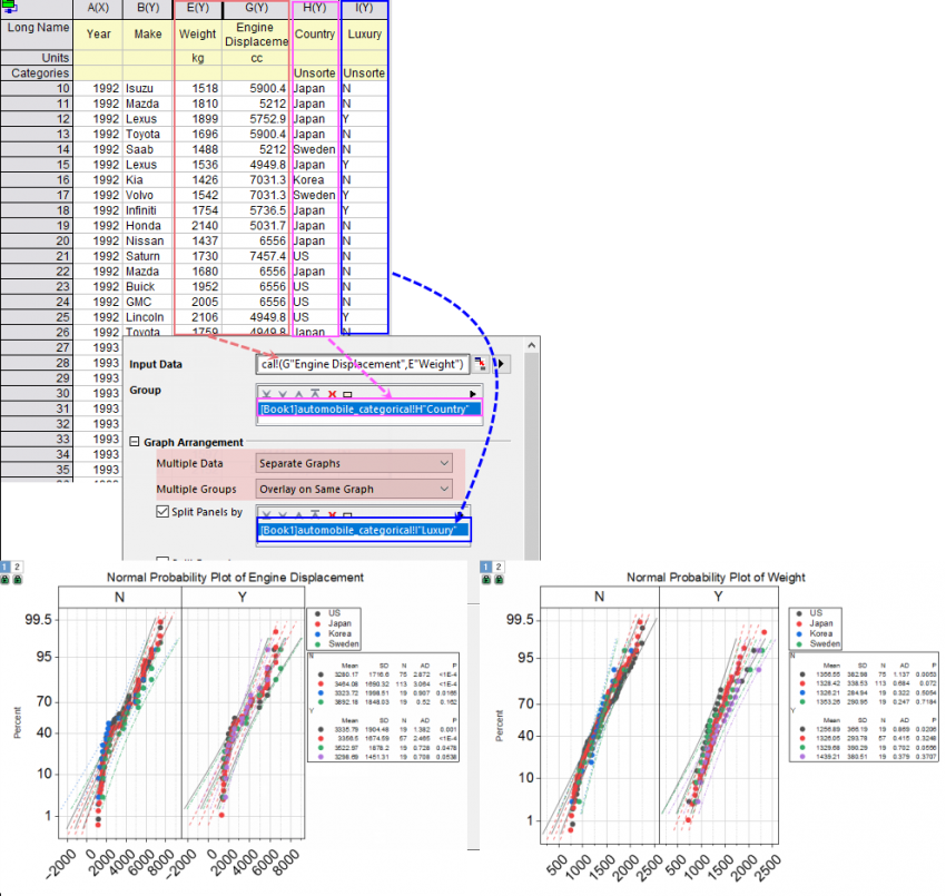
As you can see, in this example,

2 columns selected in Input Data have been plotted into separate graphs through setting Multiple Data to Separate Graphs.
The grouping column "country" selected in Group box has divided the probability plot into multiple plots overlaid on same graph.
Another grouping column "Luxury" selected in Split Panels by box has separated the graph into two layers (N and Y).
A table with statistics results have been added onto the graph.

The Dialog of plot_prob X-Function

Input Data	Specify the input data. You can select multiple columns as inout variables.
Group	Specify the grouping column(s) in order to seperate the input variable(s) into multiple different plots.
Graph Arrangement	The controls under this brach will help you arrange the multiple input variables and groups, split the graph into multiple panels and pages. Multiple Data and Multiple Groups：Use these two options , the plots will be arranged in these four ways: Overlay All: Both Multple Data and Multiple Group select Overlap on Same Graph. Overlay Groups, Variables in Different Layers: Multple Data=Separate Layers, Multiple Groups=Overlap on Same Graph Overlay Variables, Groups in Different Layers: Multiple Groups=Separate Layers, Multple Data=Overlap on Same Graph Different Layers: Both Multple Data and Multiple Groups select Separate Layers Split Panels by: Once this check box has been checked, you can select another grouping column to separate the graphs into multiple layers. Note: If Multiple Data and Multiple Groups both are set to Separate Layers, the layer order in result sheet should follow the hierarchy of "by Input Data" →"Split Panels by" → "by Groups" Split Pages by: Once this check box has been checked, you can select other grouping column(s) to split the input data and created probability plots in different graph pages. Each page only plots the columns within the same page related group. Page related group info will be shown in layer title, separated by comma if there are multiple factors. Report graph sheet will list all pages.
Share X Scales	Specify whether share X scales for all layers on same graph. This option is only available when Separate Layers on Same Graph selected in Multiple Data and Multiple Groups or grouping columns selected in Split Panels by box.
Share Y Scales	Specify whether share Y scales for all layers on same graph. This option is only available for Q-Q plot when Separate Layers on Same Graph selected in Multiple Data and Multiple Groups or grouping columns selected in Split Panels by box.
Distribution	Select a distribution type for your data. For more information about distributions, please refer to . Distribution 14 distributions are available. Estimate from Data Specify whether to estimate distribution parameters from input data. If not, parameters can be specified manually. Parameters: Unchecking the Estimate from Data box activates the Parameters boxes, where you can enter custom values to draw the curves. You can check more details about in the Distribution tab of Plot Details dialog.
Score Method	Select a method for plotting percentile approximations. For more information about methods, please refer to . Blom Benard Hazen Van der Waerden Kaplan-Meier
Confidence Band	Specify whether to output the confidence band in probability plot. For computation details, see .
Confidence Level(%)	Only available when Confidence Band is selected. Specify the confidence level in percentage for the chosen distribution.
Exchange X-Y Axes	Specify whether to switch X and Y axis positions.
X Minimum X Maximum	By default, Auto boxes are checked, which means the minimum and maximum X values of the Reference Line columns in the result sheet "PlotData#" will be used to created the distribution curves. Uncheck the Auto check box, you can enter the minimum and/or maximum of the X values for all distribution reference lines. All refence lines will be plotted within this X range.
Output To	Specify where to output the graph(s), as separate graph window(s) or embed within the report sheet.
Output Range	This determines where the calculated data for the graph is stored.
Output Graphs	This determines where the result graphs are stored.

Distributions

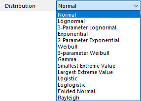
Origin includes four distributions for Probability and Q-Q plots. The following table lists their density functions:

Distribution	Density Function p(x)	Range	Parameters
Normal	\[\frac 1{\sigma \sqrt{2\pi }}\exp \left( -\frac{\left( x-\mu \right) ^2}{2\sigma ^2}\right)\]	all \(x\)	\(\mu\),mean,is the location parameter \(\sigma(>0)\),standard deviation, is the scale parameter
Lognormal	\[\frac 1{\sigma x\sqrt{2\pi }}\exp \left( -\frac{\left( \ln \left( x\right) -\mu \right) ^2}{2\sigma ^2}\right)\]	\[x>0\]	\(\mu\) is the shape scale parameter \(\sigma(>0)\) is the scale parameter.
3-parameter Lognormal	\[\frac{1}{(x - \gamma)\sigma\sqrt{2\pi}} \exp\left(-\frac{[\ln(x - \gamma) - \mu]^2}{2\sigma^2}\right)\]	\[x > \gamma\]	\(\gamma\) is Minimum value of the distribution \(\mu\) is Mean of the logarithm of (X−γ) \(\sigma >0\) is Standard deviation of ln(X−γ).
Exponential	\[\frac 1\sigma \exp \left( -\frac x\sigma \right)\]	\[x>0\]	\(\sigma(>0)\) is the scale parameter.
2-parameter Exponential	\[\lambda e^{-\lambda(x - \mu)}\]	\[x>\mu\]	λ>0 is the rate parameter (inverse scale) μ is the location parameter (minimum value, threshold).
Weibull	\[\frac c\sigma \left( \frac x\sigma \right) ^{c-1}\exp \left( -\left( \frac x\sigma \right) ^c\right)\]	\[x>0\]	\(\sigma(>0)\) is the scale parameter \(c(>0)\) is the shape parameter
3-parameter Weibull	\[\frac{k}{\lambda} \left(\frac{x - \gamma}{\lambda}\right)^{k-1} \exp\left[-\left(\frac{x - \gamma}{\lambda}\right)^k\right]\]	\[\quad x \geq \gamma\]	k>0 is the shape parameter (Weibull modulus) λ>0 is the scale parameter (characteristic life) γ is the location parameter (minimum life/threshold)
Gamma	\[\frac{1}{\Gamma(c)\sigma^c}x^{c -1} exp(-x/\sigma),\]	\[x>0\]	\(\sigma(>0)\) is the scale parameter \(c(>0)\) is the shape parameter
Smallest Extreme Value	\[\frac{1}{\sigma} \exp\left[\frac{x-\mu}{\sigma} - \exp\left(\frac{x-\mu}{\sigma}\right)\right]\]	\[\quad -\infty < x < \infty\]	μ = location parameter (mode, also median) σ>0 = scale parameter
Largest Extreme Value	\[\frac{1}{\sigma} \exp\left[-\frac{x-\mu}{\sigma} - \exp\left(-\frac{x-\mu}{\sigma}\right)\right]\]	\[-\infty < x < \infty\]	μ = location parameter (mode) σ>0 = scale parameter
Logistic	\[\frac{\exp\left(-\frac{x-\mu}{s}\right)}{s\left[1 + \exp\left(-\frac{x-\mu}{s}\right)\right]^2} = \frac{1}{4s} \text{sech}^2\left(\frac{x-\mu}{2s}\right)\]	\[ -\infty < x < \infty\]	μ = location parameter (mean, median, mode) s>0 = scale parameter (related to standard deviation)
Loglogistic	\[\frac{(\beta/\alpha)(t/\alpha)^{\beta-1}}{\left[1 + (t/\alpha)^\beta\right]^2}\]	\[t > 0\]	α>0 = scale parameter (median = α ) β>0 = shape parameter (controls skewness and tail behavior)
Folded Normal	\[\frac{1}{\sigma\sqrt{2\pi}} \left[\exp\left(-\frac{(x-\mu)^2}{2\sigma^2}\right) + \exp\left(-\frac{(x+\mu)^2}{2\sigma^2}\right)\right]\]	\[x \geq 0\]	μ is location of underlying normal σ>0 (scale)
Rayleigh	\[\frac{x}{\sigma^2} \exp\left(-\frac{x^2}{2\sigma^2}\right)\]	\[x \geq 0\]	σ>0 is the scale parameter.

Details for Constructing Probability Plot

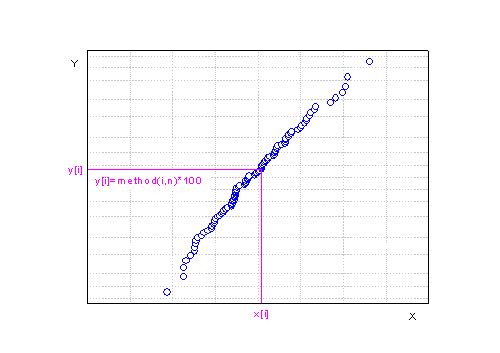
To construct a probability plot, sort the observed dataset from smallest to largest:

\(x[1]\le x[2]\le x[3]\le \cdots \le x[n-1]\le x[n]\), \(n\) is the total number of the observed dataset.

The sorted observed values are represented on the plot by points whose X-coordinates are \(x[i]\ \) and whose Y-coordinates are calculated using the .

of probability plot are different according to the distributions

Distribution	X Scale Type	Y Scale Type
Normal	Linear	Probability
Lognormal	Ln	Probability
3-parameter Lognormal	Log10	Probability
Exponential	Ln	Double Log Reciprocal
2-parameter Exponential	Log10	Double Log Reciprocal(Weibull)
Weibull	Log10	Double Log Reciprocal
3-parameter Weibull	Log10	Double Log Reciprocal(Weibull)
Gamma	Log10	Probability
Smallest Extreme Value	Linear	Double Log Reciprocal(Weibull)
Largest Extreme Value	Linear	Custom Formula
Logistic	Linear	Logit
Loglogistic	Log10	Logit
Folded Normal	Linear	Custom Formula
Rayleigh	Log10	Custom Formula

Details for Constructing Q-Q Plot

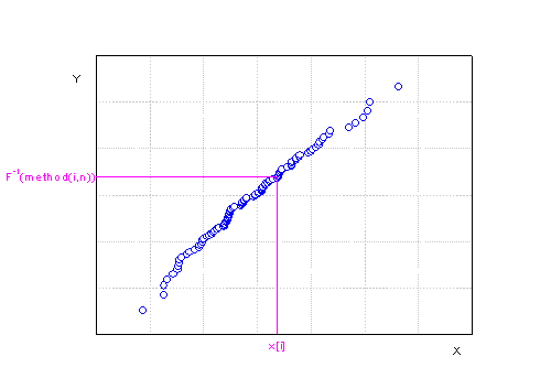
To construct a Q-Q plot,sort the observed dataset from smallest to largest:

\(x[1]\le x[2]\le x[3]\le \cdots \le x[n-1]\le x[n]\), where \(n\) is the total number of observed values.

The Y values are the inverse cumulative distribution functions of the used.

Score Methods

Input data is ordered from smallest to largest, and then the serial number of the sorted data is scored using one of the methods listed below. In this table, \(i\) is the serial number and \(n\) is the total number of the nonmissing input data.

Methods	Plotting Position \(method(i,n)\)
Blom	\[(i-0.375)/(n+0.25)\]
Benard	\[(i-0.3)/(n+0.4)\]
Hazen	\[(i-0.5)/n\]
Van der Waerden	\[i/(n+1)\]
Kaplan-Meier	\[i/n\]

Reference

Samuel Kotz , Campbell B. Read , N. Balakrishnan, Brani Vidakovic, 2005. Encyclopedia of statistical sciences., NewYork: John Wiley & Sons, Inc.
Thode, Henry C. 2002, Testing for Normality, CRC Press