16.2 Interpolate/Extrapolate Y from X

See more related video:Origin VT-0010 Interpolation

1 Overview
- 1.1 To Interpolate Y from X
2 Dialog Options
3 Algorithm
4 References

Overview

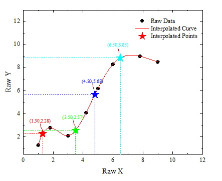
Interpolation is a method of estimating and constructing new data points from a discrete set of known data points. Given an X vector, this function interpolates a vector Y based on the input curve (XY Range). Origin provides four options for data interpolation: Linear, Cubic spline, Cubic B-spline, Akima Spline.

Linear interpolation is the simplest and fastest data interpolation method. In linear interpolation, the arithmetic mean of two adjacent data points is calculated. This method is useful in situations where low precision can be tolerated. Linear interpolation is also useful for extremely large data sets, because the calculations are not time- or computation-power intensive.

The generalization of linear interpolation is polynomial interpolation. Polynomial interpolation requires much more computation power than linear interpolation and when the polynomial order is high, the fit of the data oscillates wildly. These disadvantages can be avoided by using low-order polynomial fitting, or spline interpolation.

The Cubic spline method uses 3^rd order polynomials, and executes data-fitting in a piecewise fashion. Spline interpolation incurs less error than linear interpolation, and the interpolant is smoother.

Similar to Cubic spline interpolation, Cubic B-spline interpolation also fits the data in a piecewise fashion, but it uses 3^rd order Bezier splines to approximate the data. Cubic B-Splines allow the accurate modeling of more general classes of geometry.

To Interpolate Y from X

Create a new worksheet with input data.
Select desired data.
Select Analysis: Mathematics:Interpolate/Extrapolate Y from X. This opens the interp1 dialog.

The interp1 X-Function is called to perform the calculation.

Note: To generate uniform linearly spaced interpolated values, use the Interpolate/Extrapolate... menu command.

Dialog Options

Recalculate	Controls recalculation of analysis results None Auto Manual For more information, see: Recalculating Analysis Results
X Values to Interpolate	The X column to interpolate on.
Input	The reference XY column(s) by which to interpolate Y from specify X column. Multiple XY columns can be choosed. If multi-XY are selected, each set of XY will be used as reference to interpolate the same X column and output the corresponding Y column and the coefficient value. For help with range controls, see: Specifying Your Input Data
Method	Specify interpolation methods Linear Linear interpolation is a fast method of estimating a data point by constructing a line between two neighboring data points. The resulting point may not be an accurate estimation of the missing data. Cubic Spline This method splits the input data into a given number of pieces, and fits each segment with a cubic polynomial. The second derivative of each cubic function is set equal to zero. With these boundary conditions met, an entire function can be constructed in a piece-wise manner. Cubic B-Spline This method also splits the input data into pieces, each segment is fitted with discrete Bezier splines. Akima Spline This method is based on a piecewise function composed of a set of polynomials. The akima interpolation is stable to outliers.
Extrapolate Option	When parts of the data range specified by X Values to Interpolate is outside that of the X range specified in Input, these range parts will be considered as the extrapolated range, because the resulted Y values for these parts will be computed from extrapolation. This option can then be used to specify how to extrapolate the corresponding Y values. Extrapolate Extrapolate Y using the last two points Set missing Set all Y values in the extrapolated range to be missing values. Repeat the last value Use the Y value of the closest input X value for all values in the extrapolated range.
Boundary	Boundary condition is only available in cubic spline method. Natural 2nd derivatives are 0 on both ends. Not-A-Knot 3rd derivatives are continuous on the second and last-second point.
Smoothing Factor	Smoothing is only available in Cubic B-Spline method.
Result of interpolation	The Y column(s) to output the inteplated Y values.
Coefficients	Output the coefficients for Spline or B-spline method or not, and show them in which column.

Algorithm

Given a sequence of distinct pairs of data ( $x_i\,$ , $y_i\,$ ), where $i= 0, 1, ... n-1\!$ . we are looking for the interpolated $y\!$ at $x\!$ by the following methods:

1. Linear interpolation (interp1q)

For $x<x_{0,}y=y_0+\frac{y_1-y_0}{x_1-x_0}\times (x-x_0)$

For $x>x_{n-1,}y=y_{n-1}+\frac{y_{n-1}-y_{n-2}}{x_{n-1}-x_{n-2}}\times (x-x_{n-1})$

For $x_i<x<x_{i+1,}y=y_i+\frac{(y_{i+1}-y_{i)}}{(x_{i+1}-x_{i)}}\times (x-x_i)$

2. Cubic spline (spline)

Origin uses the natural cubic spline to do interpolation:

$y=Ay_i+By_{i+1}+Cy_i^{''}+Dy_{i+1}^{''}$

where:

$A\equiv \frac{x_{i+1}-x}{x_{i+1}-x_i},B\equiv 1-A,C\equiv \frac 16\left( A^3-A\right) \left( x_{i+1}-x_i\right) ^2,D\equiv \frac 16(B^3-B)(x_{i+1}-x_i)^2$

And $y_i^{''}$ can be generated from:

$\frac{x_i-x_{i-1}}6y_{i-1}+\frac{x_{i+1}-x_{i-1}}3y_i+\frac{x_{i+1}-x_i}6y_{i+1}=\frac{y_{i+1}-y_i}{x_{i+1}-x_i}-\frac{y_i-y_{i-1}}{x_i-x_{i-1}}$

For boundary points, we set $y_o^{''}$ and $y_{n-1}^{''}$ equal to zero.

3. Cubic B-spline (bspline)

For $x<x_0\!$ or $x>x_{n-1}\!$ perform linear interpolation.

For $x_0<x<x_{n-1},y=\sum_{i=1}^{n-4} c_iN_i(x)$

Here, $N(x)\!$ denotes the normalized cubic B-spline defined upon the knots $x_i\,$ , $x_i+1\,$ , ..., $x_i+4\,$ , And $c_i\,$ denotes the coefficient of the corresponding function.

The total number $n\!$ of these knots and their values $x_1\,$ , ..., $x_n\,$ are chosen automatically by the function. The knots $x_5\,$ , ..., $x_n-4\,$ are the interior knots; they divide the approximation interval [ $x_1\,$ , $x_m\,$ ] in to $n-7\!$ sub-intervals. The coefficients $c_1\,$ , $c_2\,$ , ..., $c_n-4\,$ are then determined as the solution of the following constrained minimization problem:

minimize

$\eta =\sum_{i=5}^{n-4}\delta _i^2\,$

subject to the constraint

$\theta =\sum_{r=1}^m\varepsilon _r^2\leq S\,$

where $\delta _i\,$ stands for the discontinuity jump in the third order derivative of $y\!$ at the interior knot $x_i\,$ , $\varepsilon _r\,$ denotes the weighted residual $w_r (y_r-y(x_r))\,$ , and S is a non-negatative number to be specified by the user.

The quantity $\eta\,$ can be seen as a measure of the (lack of) smoothness of $y\!$ , while closeness of fit is measured through $\theta\,$ . By means of the parameter $S\!$ , 'the smoothing factor', the user will then control the balance between these two (usually conflicting) properties. If $S\!$ is too large, the spline will be too smooth and signal will be lost (underfit); if $S\!$ is too small, the spline will pick up too much noise (overfit). In the extreme cases the function will return an interpolating spline ( $\theta\,$ =0) is $S\!$ is set to zero, and the weighted least-squares cubic polynomial ( $\eta\,$ =0) is $S\!$ if set very large. Experimenting with $S\!$ values between these two extremes should result in a good compromise.

4. Akima Spline (akima)

The Akima interpolation method is based on a piecewise function composed of a set of polynomials(third degree at most). This piecewise function can be applied to successive intervals of the given XY points. The slope of the input data plot at each given point can be assumed to be determined by the XY coordinates of 4 neighbor points and the point itself. Then from the slopes at two paired given points and their coordinates, a third degree polynomial is calculated, representing the interval curve between these two points, and the interpolation is then carried out based on the combination of polynomials. An additional estimation is made when calculating polynomials for end points.

Firstly the curve slope $t$ at a given point will be calculated. For a given point (point 3), there will then be five data points 1,2,3,4,5, and $m_{1}, m_{2}, m_{3}, m_{4}$ are slopes of line segments $\bar{12}, \bar{23}, \bar{34}, \bar{45}$ respectively, and $m_i=(y_{i+1}-y_i)/(x_{i+1}-x_i)$ . The curve slope $t$ is then determined by the following equations under different conditions:

When $m_{1}\neq m_{2}$ or $m_{3}\neq m_{4}$ ,

$t = \left ( \left | m_{4} - m_{3} \right |m_{2} + \left | m_{2} - m_{1} \right |m_{3} \right )/\left ( \left | m_{4} - m_{3} \right | + \left | m_{2} - m_{1} \right |\right )$

When $m_{1} = m_{2}$ and $m_{3} = m_{4}$ ,

$t = \frac{(x_4-x_3)m_2 + (x_3-x_2)m_3}{x_4-x_2}$

Slopes for two end points need to be estimated at each end of the curve. To estimate them, we calculate its slope by interpolating a parabolic curve from its adjacent three points, e.g. for the first point's slope, we can interpolate a parabolic curve from first three points, and the first point's slope can be calculated by the derivative of the interpolated curve.

Then the polynomial for an interval $[x_i, x_{i+1}]$ between two consecutive data points $\left ( x_i, y_i \right )$ and $\left ( x_{i+1}, y_{i+1} \right )$ are determined by the following four conditions: