16.7 Integrate
Math-Integrate
Description
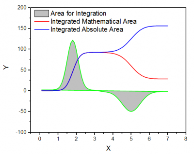
Integration tool performs numerical integration on the active data plot using the trapezoidal rule. You can choose to calculate the Mathematical Area (the algebraic sum of trapezoids) or an Absolute Area (the sum of absolute trapezoid values). Missing values are ignored.
To Use Integration Tool
- Create a new worksheet with input data.
- Highlight the selected data.
- Select Analysis: Mathematics: Integrate from the Origin menu to open the Integ1 dialog box.
The X-Function Integ1 is called to perform the calculation. The user has the option to specify that the area, peak location, peak width, and peak height (maximum deflection from the X axis), are written to the Result Log. In addition, you can choose to integrate using a simple baseline defined by a straight line connecting the end points of the curve and to create a plot of the integral curve.
 | Note: This tool uses pure, math-based integration which may produce unexpectedly negative results for area when the X values used in the integration are in descending order. This is normal behavior due to the nature of the integration calculations.
|
Dialog Options
| Results Log Output
|
Select to output area, peak location, peak width, and peak height to the Results Log.
|
| Recalculate
|
Controls recalculation of analysis results
For more information, see: Recalculating Analysis Results
|
| Input
|
Specify the input data to be integrated.
For help with range controls, see: Specifying Your Input Data
|
| Use End Points Straight Line as Baseline
|
Specify whether to create a straight line that crosses the end points and use it as the baseline for the integration.
|
| Area Type
|
Specify the integral area type. Please see the Algorithm section below, for more details.
- Mathematical Area
- The area is the algebraic sum of trapezoids.
- Absolute Area
- The area is sum of absolute trapezoid values.
|
| Output Quantities
|
Specify the quantities to be outputted when the Integration Result box is checked (see below).
- Dataset Identifier
- Choose a dataset identifier for use when the Integration Result box is checked.
- Beginning Row Index
- Specify whether to output the beginning row index.
- Ending Row Index
- Specify whether to output the ending row index.
- Beginning X
- Specify whether to output the beginning X value.
- Ending X
- Specify whether to output the ending X value.
- Max Height
- Specify whether to output the maximum height, as computed from the baseline.
- X at Max Height
- Specify whether to output the X value that corresponds to the maximum height.
- Area
- Specify whether to output the integration area.
- FWHM
- Specify whether to output the peak width at half height of the source curve.
Note: The beginning and ending X values and the integrated area are output to the Comments row of the integration results column, regardless of whether the Output Quantities Beginning X, Ending X and Area are enabled.
|
| Integral Curve Data
|
Specify the range to output the cumulative result.
|
| Integration Result
|
Specify whether output the intergration result in a report sheet.
|
| Plot Integral Curve
|
Specify whether to plot the integral curve, and where to plot the integral curve.
- None
- Do not plot the integral curve.
- New Graph
- Plot the integral to a new graph.
- Source Graph
- Plot the integral in the source graph. This option is available when a graph window is the active window.
|
| Rescale Source Graph
|
Rescale the source graph when the integral is plotted into it. This check-box is available when the Plot Integral Curve is Source Graph.
|
Algorithm
Numerical integration involves calculating a definite integral by an approximate function:
dx")
Since the original data are discrete, we use a pair of adjacent values to form a trapezoid for approximating the area beneath the segment of the curve defined by the two points:
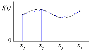
As illustrated above, the curve is divided into pieces and we calculate the sum of each trapezoid to estimate the integral by:
![\int _{x_1}^{x_n}f(x)dx \approx \sum _{i=1}^{n-1}( x_{i+1} -x_i) \frac{1}{2}[f(x_{i+1})+f(x_i)]](/origin-help/en/images/Integrate/math-02e1de68d6e5a54203ad7578c5a02844.png?v=0 "\int _{x_1}^{x_n}f(x)dx \approx \sum _{i=1}^{n-1}( x_{i+1} -x_i) \frac{1}{2}[f(x_{i+1})+f(x_i)]")
- Difference between Mathematical Area and Absolute Area
Given a baseline \!") , the mathematical area of
, the mathematical area of \!") can be calculated by
can be calculated by
![\int _{x_1}^{x_n} \left[f \left( x \right)-f \left( x_0 \right) \right] \,dx \approx \sum _{i=1}^{n-1} \frac{1}{2} \left( x_{i+1} -x_i \right) \left[ \left( f \left( x_{i+1} \right) -f \left( x_0 \right) \right) + \left( f \left( x_i \right) -f \left( x_0 \right) \right) \right]](/origin-help/en/images/Integrate/math-a25d330f4319359dc2e20213e8096e19.png?v=0 "\int _{x_1}^{x_n} \left[f \left( x \right)-f \left( x_0 \right) \right] \,dx \approx \sum _{i=1}^{n-1} \frac{1}{2} \left( x_{i+1} -x_i \right) \left[ \left( f \left( x_{i+1} \right) -f \left( x_0 \right) \right) + \left( f \left( x_i \right) -f \left( x_0 \right) \right) \right]")
If the sum of each trapezoid's area absolute value is computed, we can get the absolute area:
![\int _{x_1}^{x_n} | \left[f \left( x \right)-f \left( x_0 \right) \right] | \,dx \approx \sum _{i=1}^{n-1} \frac{1}{2} \left( x_{i+1} -x_i \right) | \left[ \left( f \left( x_{i+1} \right) -f \left( x_0 \right) \right) + \left( f \left( x_i \right) -f \left( x_0 \right) \right) \right] |](/origin-help/en/images/Integrate/math-2c032ecbce6257d0ec1dfd6f4510b0ad.png?v=0 "\int _{x_1}^{x_n} | \left[f \left( x \right)-f \left( x_0 \right) \right] | \,dx \approx \sum _{i=1}^{n-1} \frac{1}{2} \left( x_{i+1} -x_i \right) | \left[ \left( f \left( x_{i+1} \right) -f \left( x_0 \right) \right) + \left( f \left( x_i \right) -f \left( x_0 \right) \right) \right] |")
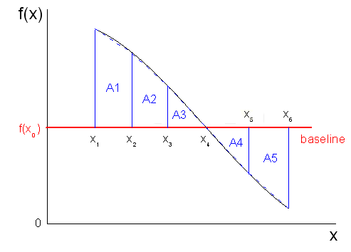
As illustrated above, the baseline is and the curve is divided into five trapezoids (or triangles). The area of each trapezoid (or triangle) is calculated by
![A_i = \frac{1}{2} \left( x_{i+1} -x_i \right) \left[ \left( f \left( x_{i+1} \right) -f \left( x_0 \right) \right) + \left( f \left( x_i \right) -f \left( x_0 \right) \right) \right]](/origin-help/en/images/Integrate/math-741a03a31a9c340fc809dbde0bfd9d03.png?v=0 "A_i = \frac{1}{2} \left( x_{i+1} -x_i \right) \left[ \left( f \left( x_{i+1} \right) -f \left( x_0 \right) \right) + \left( f \left( x_i \right) -f \left( x_0 \right) \right) \right]")
From the expression, we determine that  ,
,  and
and  , which are above the baseline, are positive, but
  and
and  , which are beneath the baseline, are negative.
So the mathematical area of this curve should be  and the absolute area of this curve should be
  .
.