17.1.1.1 The Statistics on Columns Dialog Box

1 Supporting Information
2 Recalculate
3 Input
4 Quantities
5 Computation Control
6 Output
7 Plots

Supporting Information

Recalculate

See Recalculating Analysis Results for details of the recalculation options.

Input

Exclude Empty Dataset

Check this check box to exclude empty dataset in calculation.

Exclude Text Dataset

Check this check box to exclude Text dataset in calculation.

Input Data

Specify the input data mode, indexed or raw.

Independent Columns	Each column will be treated as separate dataset. Statistical operations will be performed on each, independently.
Combined as Single Dataset	All columns will be treated as a whole.
Range1	Specify the data range to be performed: Data Range The input data range Group Multiple grouping columns contains grouping information can be inserted into the Group box. Different grouping values indicate the data in the corresponding cells are from different groups. You can add, remove, order grouping columns via controlling buttons: Move Up button , Move Down button , Remove button , Select All button , Select button in toolbar . The grouping columns are set as categorical if most of the column values are text. So you can easily reorder the output columns. Weighting Range The range that contains weighting information. The value in each cell specifies the weight of the corresponding data.

Independent Columns

Each column will be treated as separate dataset. Statistical operations will be performed on each, independently.

Combined as Single Dataset

All columns will be treated as a whole.

Range1

Specify the data range to be performed:

Data Range

The input data range

Group

Multiple grouping columns contains grouping information can be inserted into the Group box. Different grouping values indicate the data in the corresponding cells are from different groups. You can add, remove, order grouping columns via controlling buttons: Move Up button

, Move Down button

, Remove button

, Select All button

, Select button

in toolbar

.
The grouping columns are set as categorical if most of the column values are text. So you can easily reorder the output columns.

Weighting Range

The range that contains weighting information. The value in each cell specifies the weight of the corresponding data.

Quantities

Moments

Let $x_i\,$ be the $i\,$ th sample and $w_i\,$ be the $i\,$ th weight:

N Total	Total number of data points, denoted by n
N Missing	Number of missing values
Mean	The mean (average) score $\bar{x}=\frac 1w\sum_{i=1}^n x_iw_i$ . If there is no WEIGHT variable, the formula reduces to $\frac 1n\sum_{i=1}^n x_i$ .
Standard deviation	$s=\sqrt{\sum_{i=1}^n w_i(x_i-\bar{x})^2/d}$ where $d=n-1 \,$ Note: In OriginPro, $d$ has 4 more options, which are defined in the Variance Divisor of Moment branch.
SE of Mean	Standard error of mean: $\frac s{\sqrt{w}}$
Lower 95% CI of Mean	Lower limit of the 95% confidence interval of mean $\bar{x}-t_{(1-\alpha /2)}\frac s{\sqrt{n}}$ where $t_{(1-\alpha /2)}$ is the $(1-\alpha /2)$ critical value of the Student's t-statistic with n-1 degrees of freedom
Upper 95% CI of Mean	Upper limit of the 95% confidence interval of mean $\bar{x}+t_{(1-\alpha /2)}\frac s{\sqrt{n}}$ where $t_{(1-\alpha /2)}$ is the $(1-\alpha /2)$ critical value of the Student's t-statistic with n-1 degrees of freedom
Variance	$s^2\$
Sum	$\sum_{i=1}^n x_iw_i$ . If there is no WEIGHT variable, the formula reduces to $\sum_{i=1}^n x_i$ .
Skewness	Skewness measures the degree of asymmetry of a distribution. It is defined as $\gamma_1=\frac n{(n-1)(n-2)}\sum_{i=1}^n w_i^{\frac 32}(\frac{x_i-\bar{x}}s)^3 ,\mbox{for DF}$ $\gamma_1=\frac 1n\sum_{i=1}^n w_i^{\frac 32}(\frac{x_i-\bar{x}}s)^3,\mbox{for N}$ $\gamma_1=\frac 1d\sum_{i=1}^n w_i^{\frac 32}(\frac{x_i-\bar{x}}s)^3,\mbox{for WVR}$ Note: When the WDF or WS methods are chosen, skewness is returned as a missing value.
Kurtosis	Kurtosis depicts the degree of peakedness of a distribution. $\gamma_2=\frac{n(n+1)}{(n-1)(n-2)(n-3)}\sum_{i=1}^n w_i^2(\frac{x_i-\bar{x}}s)^4-\frac{3(n-1)^2}{(n-2)(n-3)},\mbox{for DF}$ $\gamma_2=\frac 1n\sum_{i=1}^n w_i^2(\frac{x_i-\bar{x}}s)^4 -3,\mbox{for N}$ $\gamma_2=\frac 1d\sum_{i=1}^n w_i^2(\frac{x_i-\bar{x}}s)^4 -3,\mbox{for WVR}$ Note: When the WDF or WS methods are chosen, kurtosis is returned as a missing value.
Uncorrected Sum of Squares	$\sum_{i=1}^n w_ix_i^2$
Corrected Sum of Squares	$\sum_{i=1}^n w_i(x_i-\bar{x})^2$
Coefficient of Variance	$\frac s{\bar{x}}$
Mean absolute Deviation	$\frac{ \sum_{i=1}^n w_i\|x_i-\bar{x}\|}w$
SD times 2	Standard deviation times 2. $2s \,$
SD times 3	Standard deviation times 3. $3s \,$
Geometric Mean	$\bar{x}_g=\left( \prod_{i=1}^n x_i\right) ^{\frac 1n}$ Note:: Weights are ignored for the geometric mean.
Geometric SD	The geometric standard deviation $e^{std(\log x_i)}$ Where std is the unweighted sample standard deviation. Note: Weights are ignored for the geometric standard deviation.
Mode	The mode is the element that appears most often in the data range. If multiple modes are found, the smallest will be chosen.
Sum of Weights	$w=\sum_{i=1}^n w_i$
Harmonic Mean	harmonic mean (sometimes called the subcontrary mean) without weight: $\frac n{\frac 1{x_1} + \frac 1{x_2} + ... + \frac 1{x_n}}=\left(\frac {\sum_{i=1}^n (x_i)^{-1}}n\right)^{-1}$ with weight: $\frac {\sum_{i=1}^n w_i}{\sum_{i=1}^n \frac {w_i}{x_i}}=\left(\frac {\sum_{i=1}^n w_i x_i^{-1}}{\sum_{i=1}^n w_i}\right)^{-1}$ if any $x_i$ or weight is negative, return missing; if any $x_i$ or weight is 0, return 0.

Quantiles

Quantiles are values from the data, below which is a given proportion of the data points in a given set. For example, 25% of data points in any set of data lay below the first quartile, and 50% of data points in a set lay below the second quartile, or median.

Sort the input dataset in ascending order. Let $x(i)\,$ be the $i\,$ th element of the reordered dataset

Minimum	$x_{(1)}\,$
Index of Minimum	The index number of Minimum in the original (input) dataset
1st Quartile (Q1)	First (25%) quantile, Q1. See Interpolation of quantiles for computational methods
Median	Median or second (50%) quantile, Q2. See Interpolation of quantiles for computational methods
3rd Quartile (Q3)	Third (75%) quantile, Q3. Interpolation of quantiles for computational methods
Maximum	$x_{(n)}\,$
Index of Maximum	The index number of Maximum in the original (input) dataset
Interquartile Range (Q3-Q1)	$Q_3-Q_1\,$
Range (Maximum-Minimum)	Maximum - Minimum
Custom Percentile(s)	Request computation of custom percentiles.
Percentile list	This option is only available when Custom Percentile(s) is checked. Percentiles are computed for all the values listed.
Median Absolute Deviation	For a univariate data set X1, X2, ..., Xn, the MAD is defined as the median of the absolute deviations from the data's median: $MAD = median(\|{X_i} - median(X)\|)\,$ that is, starting with the residuals (deviations) from the data's median, the MAD is the median of their absolute values.
Robust Coefficient of Variation	$(MAD/norminv(0.75))/Median\,$

Extreme Values

Return extreme values. Extreme values are the lst highest and the lst lowest values.
$l = \begin{cases} 5,& \mbox{if }\ n\geq 10 \\ n/2, & \mbox{otherwise } \end{cases}$

where n is the length of the dataset.

Computation Control

Weight Method

Choose weighting methods for input data.

Direct Weighting	$w_{i}=c_{i}\,\!$ , where $c_{i}\,\!$ is the ith value of weighting dataset.
Instrumental	$w_{i}=\frac 1{\sigma _{i}^2}\,\!$ , where $\sigma_{i}\,\!$ is the value in a designated error bar column.
Statistical	$w_{i}=\frac 1{x_{i}}\,\!$ , where $x_{i}\,\!$ is the input data.

Variance Divisor of Moment

Controls computation of variance divisor d.

DF	Degrees of freedom $d=n-1\,$
N	Number of non-missing observations $d=n\,$
WDF	Sum of weights DF $d=w-1\,$
WS	Sum of weights $d=w\,$
WVR	$d=w-\sum_{i=1}^n w_i^2/w$

Interpolation of quantiles

Methods for calculating Q1, Q2, and Q3:

Let the $i\,$ th percentile be y, set $p=i/100\,$ , and let

$\begin{cases} (n+1)p=j+g, & \mbox{for Weighted Average Right } \\ np=(j+g),& \mbox{for other methods } \end{cases}$

where j is the integer part of np, and g is the fractional part of np, then different methods define the $i^{th}\,$ percentile, y, as described by the following:

Empirical Distribution with Averaging	$y = \begin{cases} \frac 12(x_{(j)}+x_{(j+1)}),& \mbox{if }\ g=0 \\ x_{(j+1)},& \mbox{if }\ g>0 \end{cases}$
Nearest Neighbor	Observation numbered closest to $np\,$ $y = \begin{cases} x_k,& \mbox{if }\ g\neq \frac 12 \\ x_j, & \mbox{if }\ g=\frac 12 \mbox{ and j is even} \\ x_{(j+1)},& \mbox{if }\ g=\frac 12 \mbox{ and j is odd} \end{cases}$ where k is the integer part of $np+\frac 12\,$
Empirical Distribution	$y= \begin{cases} x_{(j)}, & \mbox{if }\ g=0 \\ x_{(j+1)},& \mbox{if }\ g>0 \end{cases}$
Weighted Average Right	weighted average aimed at $x_{((n+1)p)}\,$ $y=(1-g)x_{(j)}+gx_{(j+1)}\,$ where $x_{(n+1)}\,$ is taken to be $x_{(n)}\,$
Weighted Average Left	weighted average aimed at $x_{(np)}\,$ $y=(1-g)x_{(j)}+gx_{(j+1)}\,$ where $x_0\,$ is taken to be $x_1\,$
Tukey Hinges	Let: $m = \begin{cases} \frac n2,& \mbox{if n is even} \\ \frac{(n+1)}2,& \mbox{if n is odd} \end{cases}$ $k = \begin{cases} \frac m2,& \mbox{if m is even} \\ \frac{(m+1)}2,& \mbox{if m is odd} \end{cases}$ Then we have: $Minimun=x_{(1)}\,$ $Q_1= \begin{cases} x_k,& \mbox{if m is odd} \\ \frac 12(x_{(k)}+x_{(k+1)}),& \mbox{if m is even} \end{cases}$ $Q_2= \begin{cases} x_m,& \mbox{if n is odd} \\ \frac 12(x_{(m)}+x_{(m+1)}),& \mbox{if n is even} \end{cases}$ $Q_3= \begin{cases} x_{(n-k-1)},& \mbox{if m is odd} \\ \frac 12(x_{(n-k)}+x_{(n-k+1)}),& \mbox{if m is even} \end{cases}$ $Maximum=x_{(n)}\,$

Note: if weights are specified, Weighted Percentiles are calculated. The pth weighted percentile y is computed from the Empirical Distribution Function with Averaging: $y= \begin{cases} \frac 12(x_{(i)}+x_{(i+1)}),& \mbox{if } \sum_{j=1}^i w_j=pw \\ x_{(i+1)},& \mbox{if } \sum_{j=1}^{i} w_j<pw<\sum_{j=1}^{i+1}w_j\\ x_{(1)},& \mbox{if } \ pw<w_1 \\ x_{(n)},& \mbox{if } \ pw<w_n \\ \end{cases}$

Output

Beginning with Origin 2022, input column Format of a Group column will be preserved in the output sheet (e.g. DescStatsQuantities). For instance, when outputting stats on a column of Date-Time data, column Format will be set as Date-Time in the output sheet (previously, the column would have been formatted as Text). You can restore the old behavior by setting @SCCSF = 0. For information on changing the value of a system variable, see FAQ-708 How do I permanently change the value of a system variable?

Graph	Control arrangement of resulting plots. Arrange Graphs into Columns Specify number of columns to arrange output graphs. Arrange Plots of Same Type in One Graph Check to plot all graphs of same type in one graph window.
Dataset Identifier	Choose an identifier for the source datasets. Identifier Select from the list: Range Use the range syntax. Book Name Use the workbook long name. Sheet Name Use the worksheet name. Name Use column Long Name if it exists, otherwise Short Name. Short Name Use column Short Name. Long Name Use column Long Name. Units Use column Units. Comments Use column Comments. <Custom> Use custom formats to define a data identifier. For usage information, please refer to Advanced legend text customizations. Show Identifier in Flat Sheet Use the dataset identifier in resulting flat sheet(s).
Report Tables	Destination for report worksheet tables. Book The target workbook. <none>: Do not output report worksheet tables. <source>: The source data workbook. <new>: A new workbook. <existing>: An existing workbook. BookName The target workbook. Must be source (uneditable), new or existing (editable), otherwise blank. Sheet The target worksheet, always <new>. SheetName Name of the target sheet. Results Log Output the report to the Results Log. Script Window Output the report to the Script Window. Notes Window Specify the target Notes window: <none>: Do not output to a Notes window. <new>: Output to a new Notes window.
Quantities	Specifies the destination of quantities Book Specifies the destination workbook <none>: Do not output quantities <source>: The source data workbook <report>: The Report Tables workbook <new>: A new workbook. <existing>: A specified existing workbook BookName The target workbook. Must be source (uneditable), new or existing (editable), otherwise blank. Sheet <new>: A new worksheet. <source>: The source data worksheet <existing>: A specified existing worksheet SheetName Name of the target sheet.
Optional Report Tables	Specifies what is output to report worksheet Notes Notes table Input Data Table for input data Masked Data Table for masked data Missing Data Table for missing data

Plots

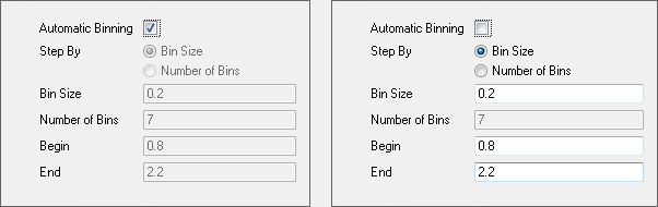
Histograms

Outputs a histogram to the result sheet.

When this box is selected, the branch is expanded. In this branch,

The Data Height drop-down determines the Y axis of the histogram.

Count: Y axis displays bin counts.
Relative Frequency: Y axis displays individual bin counts divided by total count.
Density: Y axis displays relative frequency (no. of observations in a given bin) divided by bin width.

The Automatic Binning check box is selected by default. Bin Size, Number of Bins, Begin, End are shown automatically when Automatic Binning is clear.

Note: If the input data are in multiple columns, Automatic Binning will use independent settings for each column and thus the binning and axis range may vary a lot. In this case, Origin will display non-editable limit values for each column. If the Automatic Binning check box is cleared, these items will be editable with an initial value.

After you edit the value of Bin Size, Beginning and/or End, the Number of Bins will be computed automatically.

Number of Bins and Bin Size can be switched by Step By.

Number of Bins = (Begin - End) / Bin Size

Box Charts

Outputs a box chart to the report sheet. If the input data has a group column, the box chart is grouped accordingly. If the group column is Set as Categorical, the box chart will be plotted according to categorical order customized through (Column Properties) Categories tab from grouping range.