29.1 Data Table

To create a new data table,

Click New Data Table button on the Standard toolbar,

Or,

Right click empty place inside Origin workspace and select New Data Table,

Or,

Select menu File: New: New Data Table.

1 Table Types
2 Basic Manipulates

Table Types

Free Form (Worksheet)

classic Origin worksheet. No structure. Refer to this page for detailed informatioin.

XY

This table type follows the XYYY... structure: one single X column paired with multiple Y columns. It can include an optional Row Title column (Text column for labeling rows) and an X Error column. Each Y Dataset represents a distinct group with multiple Replicates.

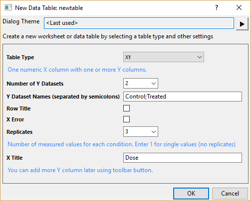
Data Format	Select the table data format: Raw Data Summary (Mean) Summary (Meadian)
Number of Groups (Y Datasets)	Select or enter the number of groups to compare. Each Y dataset has the same number of replicate columns. Note: You can add or remove datasets anytime after creating the table. To reconstruct groups and replicates, click on table icon and select Restructure Table menu. See this section for details. To insert a new Y dataset before an existing one, right click on the dataset title bar and select Insert. To delete a Y dataset, right click on the dataset title bar and select Delete.
Group Names	Enter semicolon-separated names for groups (Y datasets).
Row Title	Select this checkbox to add a Text column for row labels.
X Error	Select this checkbox to add an error bar column for X.
Replicate Values per Group	Select or enter the number of replicate sub-columns per Y dataset. Enter 1 for no replicates. Note: You can add or remove a sub-column anytime after creating the table. To add a sub-column, click Add New Columns button . New replicate is added to all datasets with the same Name. To insert a sub-column, click the Name cell of a sub-column to select that replicate, right click and select Insert. New replicate is added to all datasets in the same position. To delete an existing sub-column from all datasets, click the Name cell of a sub-column to select that replicate, right click and select Delete.
X Title	Label used for X column title.

XY tables are widely used in experiment data such as dose-response or inhibition assays where you have one measured variable and multiple outcomes in response.

Column

This table type follows the YYY... structure: multiple Y columns and no X column. Each Y column represents an independent group, and replicates are arranged in each column. It can include an optional Row Title column (Text column for labeling replicates)

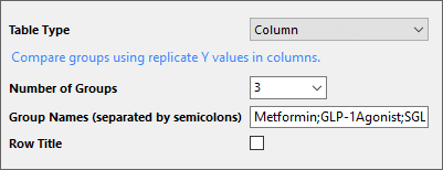
Number of Groups	Select or enter the number of groups to compare. One Y column per group. Note: You can add or remove Y columns anytime after creating the table. To add a Y column, click Add New Columns button . To insert a new column before an existing one, right click on the dataset title bar and select Insert. To delete a column, right click on the column title bar and select Delete.
Group Names	Enter semicolon-separated names for groups (Y columns).
Row Title	Select this checkbox to add a Text column for row labels.

Number of Groups

Select or enter the number of groups to compare. One Y column per group.

Note: You can add or remove Y columns anytime after creating the table.

To add a Y column, click Add New Columns button .
To insert a new column before an existing one, right click on the dataset title bar and select Insert.
To delete a column, right click on the column title bar and select Delete.

Group Names

Enter semicolon-separated names for groups (Y columns).

Row Title

Select this checkbox to add a Text column for row labels.

Column tables are mainly used for One Way ANOVA raw data and other analyses comparing independent groups measured on the same variable (e.g., t-tests, nonparametric tests).

Grouped

This table type follows the Row Titles + Y columns structure: a Title column for row labels, followed by multiple Y columns organized into Groups. Each Group represents a level of Factor A, and the Y columns within each Group represent the levels of Factor B.

You can optionally enable Subgroups to add the third factor for Three Way ANOVA. Subgroups divide each Group (Factor A) into additional levels that represent Factor B, while the Y columns within each Subgroup represent Factor C.

Note that all factors (Two way and Three way) are crossed (all combinations present).

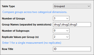
New Data Table Grouped Two Way dialog.png

Number of Groups	Select or enter the number of groups to compare across two (or three) categorical dimensions. Note: You can add or remove groups anytime after creating the table. To reconstruct groups and replicates, click on table icon and select Restructure Table menu. See this section for details. To insert a new group before an existing one, right click on the dataset title bar and select Insert. To delete a group, right click on the group title bar and select Delete.
Group Names	Enter semicolon-separated names for groups.
Number of Subgroups	For three-way ANOVA, select or enter the Number of Subgroups rather than 0 to add the third factor. Subgroups divide each Group into additional levels that represent Factor B, while the Y columns within each Subgroup represent Factor C. This creates a three-factor crossed design where Factor A (Groups), Factor B (Subgroups), and Factor C (Y columns) are all crossed with each other.
Replicate Values per Group	Select or enter the number of replicate Y columns per group. Enter 1 for no replicates. Note: You can add or remove a Ycolumn anytime after creating the table. To add a Y column, click Add New Columns button . New replicate is added to all groups with the same Name. To insert a Y column, click the Name cell of a Y column to select that single column, right click and select Insert. New replicate is added to all groups in the same position. To delete an existing Y column from all groups, click the Name cell of a Y column to select that single column, right click and select Delete.
Row Title	Select this checkbox to add a Text column for row labels.

Grouped tables are mainly used for two-way ANOVA and analyses with two independent categorical variables (factors). Each factor has two or more levels.

Contingency

This table type follows a two-way contingency structure: one Text column for row category labels, paired with multiple Numeric columns containing frequency counts. The first Text column contains labels for the first categorical variable. The following Numeric columns contain integer counts for each level of the second categorical variable.

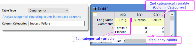
Column Categories	Enter semicolon-separated labels for the second categorical variable.

Contingency tables are designed for categorical data analysis such as chi-square tests and Fisher's exact test.

Survival

This table type follows the Time + Status structure: one X column for elapsed time, paired with one or more Y columns for event status. The X column contains the "Elapsed Time" from start of observation until event or censoring. Y columns contain "Status" indicating whether an event occurred: typically 0 = Censored (no event/withdrawn), 1 = Event (death/failure/specified outcome occurred). An optional Row Title column can be added for individual subject labels.

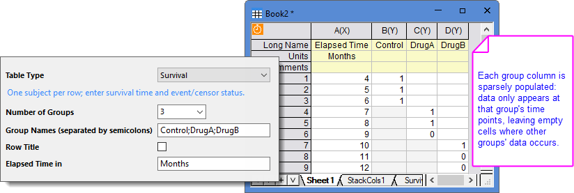
Number of Groups	Select or enter the number of groups for comparison. One Y column per group. Note: You can add or remove groups (Y columns) anytime after creating the table. To add a Y column, click Add New Columns button . To insert a new column before an existing one, right click the dataset and select Insert. To delete a column, right click the column and select Delete.
Group Names	Enter semicolon-separated names for Y columns.
Row Title	Select this checkbox to add a Text column for subject labels.
Elapsed Time in	By default, the unit of “Elapsed Time” (X column) is “Days”. Use this editbox to change the unit, Months, Years, etc.

Survival table is designed for survival analysis and reliability studies. For Kaplan-Meier estimator, quick access is available: left-clicking on the table icon (at the top-left corner) and select Kaplan-Meier Estimator... menu.

Basic Manipulates

Click the table icon at the top-left corner of the table, a list of menus pops up providing quick access to frequently used operations:

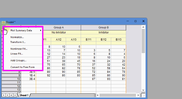
Available menus vary by table typs.

Summary Data & Plot Summary Data

Choose to plot statistics summary data with Scatter, Line, Line + Scatter, or Column charts. Y values can be Mean, Median and Geometric Mean, with optional error bars from Standard Deviation, SEM (SE of Mean), 95% CI (Upper 95% CI of Mean - Lower 95% CI of Mean), or Range (Max-Min).

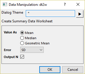
The summary data is output to a "Summary Stats" worksheet. You can also choose to output the total number N.

Normalize

Rescale data to a common relative scale, 0% to 100% or 0.0 to 1.0, for comparison across groups or subcolumns.

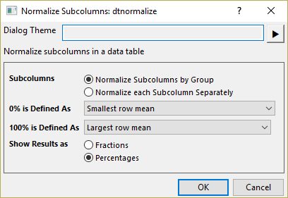
Subcolumns	Specify how to treate subcolumns in the groups when normalize. Normalize Subcolumns by Group: Normalize all subcolumns within each group together, using group-level statistics (row means). Normalize each Subcolumn Separately: Normalize each subcolumn individually using its own values.
0% is Defined As	Specify how to define 0%: If Normalize Subcolumns by Group, choose to define 0% as Smallest row mean, First row mean (or last, whichever is smaller), or Fixed value specified in 0% Fixed At edit box. If Normalize each Subcolumn Separately, choose to define 0% as Smallest value in each subcolumn, First value in each subcolumn (or last, whichever is smaller), or Fixed value specified in 0% Fixed At edit box.
100% is Defined As	Specify how to define 100%: If Normalize Subcolumns by Group, choose to define 100% as Largest row mean, Last row mean (or first, whichever is larger), Fixed value specified in 0% Fixed At edit box, Sum of all row means, or Average of all row means. If Normalize each Subcolumn Separately, choose to define 100% as Largest value in each subcolumn, Last value in each subcolumn (or first, whichever is larger), Fixed value specified in 100% Fixed At edit box, Sum of values in each subcolumn, or Average of values in each subcolumn.
Show Results as	Specify output format of normalized data. Fractions: decimal value from 0.0 to 1.0 Percentages: percentages from 0% to 100%

Transform X

Transform concentration values (X data) for dose-response analysis. This is typically a required preprocessing step for sigmoidal dose-response curve fitting.

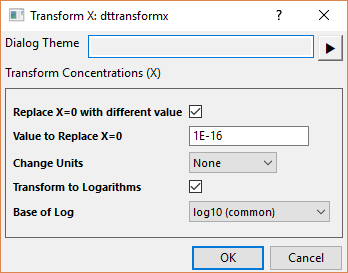
Replace X=0 with different value	If X contains zero concentrations (e.g., vehicle controls), check this checkbox to substitute "0" with a specified small value. Required before log transformation, as log(0) is undefined. Enter the replacement value in the Value to Replace X=0 edit box. A common practice is to replace 0 with 1/10 of the lowest non-zero concentration.
Change Units	Convert concentration units by multiplication or division. Select None for no units conversion. If Multiply or Divide is selected, enter the factor in the Constant to Apply edit box. For example, to convert "uM" to "mM", select Divide and 1000 in Constant to Apply.
Transform to Logarithms	Convert linear X values to log scale for sigmoidal curve fitting. Select the logarithm from Base of Log drop-down: log10 (base 10), ln (base e), and log2 (base 2).

Nonlinear Fit

Perform nonlinear curve fitting on XY data. The Nonlinear Curve Fit dialog will open, giving you full control over the fitting process.

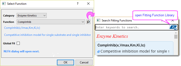
Select Function	Refer to this page for full info. about fitting Function (although the available Category may differ from the default mode). Click button to search the function you need. To access the full set of fitting functions, switch to the default mode (Preferences: GUI Mode: default) and restart Origin.
Fitting Method	Specify whether to fit using Raw Data or summary statistics: Mean + SD (SD used as weight), Mean + SE (SE used as weight), or Mean only. If summary statistics is selected, a "Summary Stats" worksheet is auto-generated to use as input data.
Global Fit	Check this checkbox to share parameters in the fitting function among all datasets (groups), yielding the same parameter values for all datasets. Uncheck to fit each dataset independently and yield separate results for each dataset (although they will be compiled into a single report). Refer to this page for details about Global Fit.

Select Function

Refer to this page for full info. about fitting Function (although the available Category may differ from the default mode). Click

button to search the function you need.

To access the full set of fitting functions, switch to the default mode (Preferences: GUI Mode: default) and restart Origin.

Fitting Method

Specify whether to fit using Raw Data or summary statistics: Mean + SD (SD used as weight), Mean + SE (SE used as weight), or Mean only. If summary statistics is selected, a "Summary Stats" worksheet is auto-generated to use as input data.

Global Fit

Check this checkbox to share parameters in the fitting function among all datasets (groups), yielding the same parameter values for all datasets.

Uncheck to fit each dataset independently and yield separate results for each dataset (although they will be compiled into a single report).

Refer to this page for details about Global Fit.

Linear Fit

Perform linear regression on XY data. Each group is fitted independently, and all fitting results are compiled into a single report. The Linear Fit dialog will open, giving you full control over the fitting process.

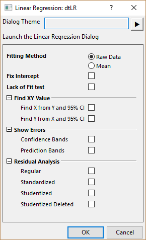
Fitting Method	Specify whether to fit with original data or summary data. Raw Data Each group is fitted independently. Replicates within each group are concatenated and fitted as one dataset. Mean A "Summary Stats" worksheet is auto-generated to calculate the mean of replicates within each group. Each group is then fitted independently using mean as input. Mean + SD A "Summary Stats" worksheet is auto-generated to calculate the mean and standard deviation of replicates within each group. Each group is then fitted independently using its mean as input, with the inverse of the variance (1/SD^2) as weight.
Fix Intercept	Restrict the intercept to the value specified in Fix Intercept at.
Lack of Fit test	Check to output the "Lack-of-Fit" results for replicate data, which is used to assess the model adequacy. Refer to this page for more info.
Find XY Value	Check to generate "FindXfromY" and/or "FindYfromX" worksheets: enter an independent variable value to obtain the corresponding dependent variable value, or vice versa. The 95% Confidence Interval is also calculated in the sheet. Refer to this page for more info.
Show Errors	Check to add confidence bands and/or prediction bands to the fitted curve plot. Refer to this page for more info.
Residual Analysis	Check to calculate and output residuals. Refer to this page for more info.

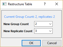
Restructure Table

Restructure data table, i.e. add or remove groups or replicates.

Convert to Free Form

Convert current data table into typical Origin worksheet form.