18.12.1.2 Algorithms (Continuous Wavelet Transform)

Continuous Wavelet Transform

This function computes the real continuous wavelet coefficient for each given scale presented in the Scale vector and each position b from 1 to n, where n is the size of the input signal.

Let x(t) be the input signal and ψ be the chosen wavelet function, the continuous wavelet coefficient of x(t) at scale a and position b is:

\[C_{a,b} = \int_R {x(t)\frac{1}{{\sqrt a }}\psi^* } (\frac{{t - b}}{a})dt\]

The computation is implemented with a NAG function: nag_cwt_real(). It does not compute the coefficients with the definition of CWT. Instead, the integrals of the scaled, shifted wavelet function are approximated and the convolution is then computed.

Origin Wavelet Types

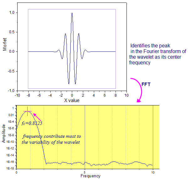
• Morlet

  The Morlet wavelet:

  \[\psi (x) = \pi ^{ - 1/4} \cos (kx)e^{ - x^2 /2}\]

  where k is the wave number.

• DGauss

  The Derivative of a Gaussian wavelet, which is the pth derivative of the Gaussian function:

  \[\psi (x) = (\frac{2}{\pi })^{ - 1/4} e^{ - x^2 }\]

  where p is the derivative order.

• MexHat

  The Mexican Hat Wavelet:

  \[\psi (x) = \frac{2}{{\sqrt 3 }}\pi ^{ - 1/4} (1 - x^2 )e^{ - x^2 /2} \]

Convert Scale to Pseudo Frequency

For a given wavelet, you can map a scale and convert to pseudo-frequency by ways below:

\[F_a=\frac{F_c}{s\cdot \Delta }\]

In this formula:

• s is a scale.
• \(\Delta\) is the sampling period.
• \(F_c\) is the center frequency of a wavelet in Hz.
• \(F_a\) is the pseudo-frequency corresponding to the scale a, in Hz.

The \(F_c\) is the frequency contributes most to the variability of the wavelet, and it can be derived from maximizing the FFT of the wavelet modulus.