Origin supports multiple Conditional Format tools to color the cells in the worksheet.
To open the dialog:
or
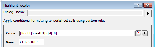
In these dialogs of the tools, you can specify Range of the cells in the worksheet and Name for the selected range.
By default, the Name is first cell-last cell of the range. For example: if the range is from Column1 Row5 to Column4 Row10, the name will be C1R5-C4R10. Also, you can define the name by entering text. And in the same Worksheet, the name of Conditional Format that have been used will list in this drop-box.
Note: for a worksheet, if you have added a Conditional Format, these tools dialog can support to update the rule, but not support to change the data range with the original Name. If you want to just update the range of the Conditional Format, you need to edit it in the Conditional Format Manager
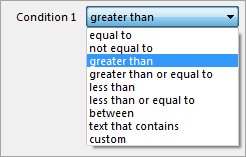
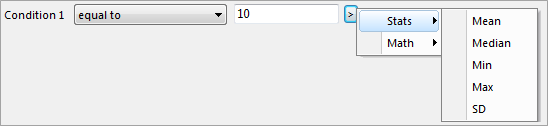
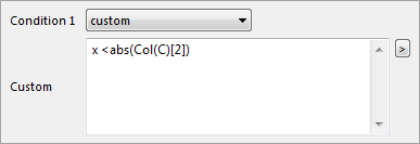
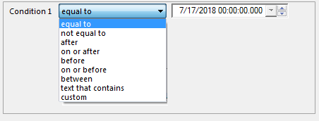
Color cells that matchs the condition setting in the dialog.
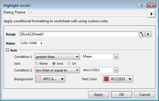
| Condition | When the range (columns) Format = Numeric
|
|---|---|
| Join | The default state is None but you can set the drop-down to either And or Or and create a second condition. |
| Background | Specify the background color for the cells value matching the conditions of the rule. |
| Text Color | Specify the text color for the cells value matching the conditions of the rule. |
Use this tool to color cells with duplicate value.
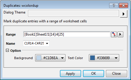
| Backgroud | Specify the backgroud color for the cells with duplicate value. |
|---|---|
| Text Color | Specify the text color for the cells with duplicate value. |
Color top/bottom N values in the selected colulmns.
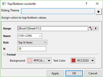
| Top N Iterms | Color the top N values in Range columns. |
|---|---|
| Top N% | Color the top N% values in Range columns. |
| Bottom N Items | Color the bottom N values in Range columns. |
| Bottom N% | Color the bottom N% values in Range columns. |
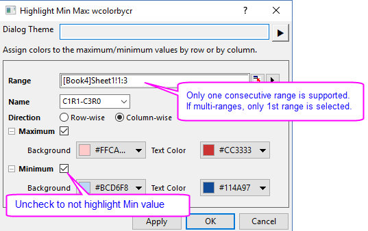
Color minimumn and/or maximum values in each selected colulmn/row, independent of other columns or rows.
Calculate count of all items in the selected range, and order them from top frequent to least frequent like Pareto chart.
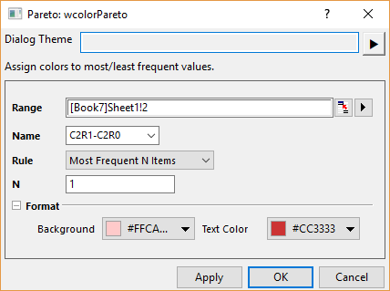
| Most Frequent N Iterms | Color the top N items of count. |
|---|---|
| Most Frequent N% | Color the items with cumulative frequency <=N%. |
| Least Frequent N Items | Color the bottom N items of count. |
| Least Frequent N% | Color the items with cumulative frequency >=(1-N%). |
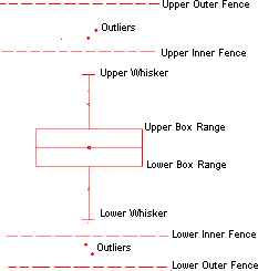
Color outliers from the selected Range like Box chart.
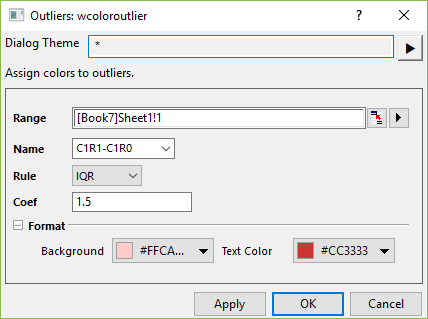
| IQR | Same as Whisker Range = Outlier in Box chart.
Select or type a value n into the Coef combo box to expand the whisker by a factor of n. With the default Coef value of 1.5, whisker length will be determined by the outermost data point that falls within upper inner and lower inner fence (a Coef = 3 would be determined by the outermost data point that falls within the upper outer and lower outer fences).
|
|---|---|
| SD | Same as Whisker Range = SD in Box chart.
Select or type a value n into the Coef combo box to expand the whisker by a factor of n. |
Use heatmap to color cells according to the level setting.
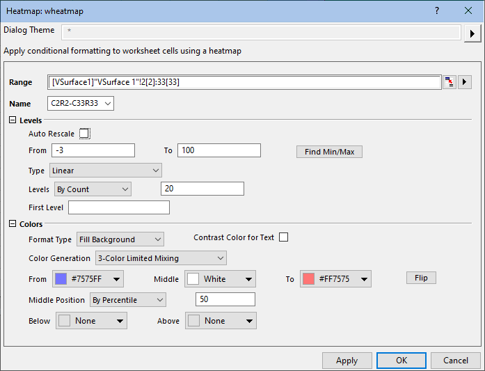
| Auto Rescale | Select this check box to auto detect automatically the maximum and minimum value of the range. By defualt, it is checked. |
|---|---|
| From | This is available only when Auto Rescale is unchecked. Use it to specify the minimum value. |
| To | This is available only when Auto Rescale is unchecked. Use it to specify the maximum value. |
| Find Mi/Max | Click this button to detect the maximum and minimum value based on the selected data range, and automatically set the To and From values. |
| Type | Select a type for the level scale. Please see details about the scale type here. |
| Levels |
|
| First Level | Specify the value of the first level. Note: this value should be larger than or equal to the default value of the first level. |
| Format Type |
Use the color to Fill Background or Color Text of the cells in the selected range. |
|---|---|
| Contrast Color for Text | Against the background color of the cells, use the contrast color for the text |
| Color Generation |
|
| From | This is available only when either Limited Mixing, 3-Color Limited Mixing or Introducing Other colors in Mixing is selected. Use it to specify the color for the minimum level. |
| Middle | This is available only when 3-Color Limited Mixing is selected. Use it to specify the color for the middle level. |
| To | This is available only when either Limited Mixing, 3-Color Limited Mixing or Introducing Other colors in Mixing is selected. Use it to specify the color for the maximum level. |
| Middle Position |
Used to control values associated with Middle color in 3-Color Limited Mixing:
|
| Palette | This is available only when Load Palette is selected. Select the built-in Increment list or Palettes. |
| Flip | Flip the order of colors for From' and To or in the selected palette. |
| Below | Specify a color and it will be used to the cell that the value less than From value. |
| Above | Specify a color and it will be used to the cell that the value greater than To value. |
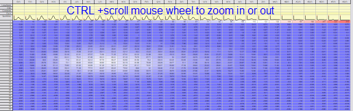
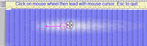
It can be handy to zoom or pan the Conditional Heatmap:
|
There are two methods to remove the Conditional Format:
The Conditional Format Manager dialog lists all the Conditional Formats in active worksheet, and it is used to manage the conditional format by editing, reordering and remove them.
To open the dialog: Worksheet: Conditional Formatting: Conditional Format Manager
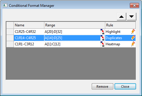
To change the Name:
Double click on the cell of the Name for the Conditional Format to rename it.
To change the Range:
or
To update the Rule:
If the range are overlapping in two Conditional Formats, the new added Conditional Format shows in upper of this list. And in the overlapping range of the worksheet will be applied the format of the upper .
To Reorder the Conditional Format:
or
Select the row of Conditional Format in the list, and click Remove button to delete the format control.