4.5.3 Signal Processing

Signal-Processing

Smoothing Plotted Datasets

This example smooths all plotted data in the active graph layer. The smoothed data is put into a new book.

// Count the number of data plots in the layer 
//and save result in variable "count"
layer -c; 
string gname$ = %H;   // Get the name of this Graph page
// Create a new book named smooth 
//actual name is stored in bkname$
newbook na:=Smoothed; 
wks.ncols=0;          // Start with no columns
loop(ii,1,count) {
    // Input Range refers to 'ii'th plot
    range riy = [gname$]!$(ii);    
    // Output Range refers to two, new columns            
    range roy = [bkname$]!($(ii*2-1),$(ii*2));
   // Savitsky-Golay smoothing using third order polynomial 
    smooth iy:=riy meth:=sg poly:=3 oy:=roy;   
}

Finding Envelopes (Pro Only)

The following script uses the envelope X-Function to find the lower and upper envelope of a signal.

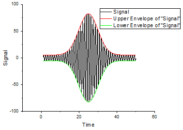
//Import a signal with Gaussian envelope
fname$ = system.path.program$ + "samples\signal processing\Gaussian Envelope.dat";
impasc;
envelope iy:=col(2) type:=both;
//Plot
plotxy iy:=(?,1:6) plot:=200;

FFT on Data with Missing Values

FFT in Origin requires that input data does not have missing values. So before you can perform FFT on data with missing values, you will need to fill in those missing data. The simplest would be to interpoate with good data nearby, using simple linear interpolation.

This example plots two different FFT Amplitudes from two date ranges of sunspot data to illustrate the ~11 year sunspot cycle, with missing data replaced by linear interpolation.

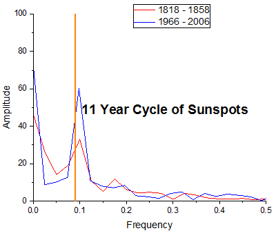
// Import the data
string fname$ = system.path.program$ + "Samples\Signal Processing\dayssn.dat";
//col(1) = year, col(2)=month, col(3)=day, 
//col(4) = date values in contiguous year with fractions
//col(5) = observation
//so we should have a sheet with 5 col and col(4)=X col(5)=Y
newbook s:=0;newsheet cols:=5 xy:="NNNXY"; 
impasc;

// Interpolate to replace missing values and put result to col(6)
interp1q 4 (4,5) 6;
// this is our data
range rData1 = 6[1:14609];// row range for years 1818 to 1858
range rData2 = 6[54057:end];// row range for years 1966 - 2006
// now start the FFT with the fft1 X-Function 
// which will create a ReportData sheet and a ReportTable sheet
fft1 rData1;
//after running an XF, a tree with same name is created, 
//here we will make use of fft1.rd the ReportData node
range rReportData1=fft1.rd$;//range to hold the Report Data from the FFT result
range rAmp1=%(rReportData1.getlayer()$)col(Amplitude);
rAmp1[C]$="1818 - 1858"; // change the Comment to make better legend for the graph

fft1 rData2;
range rReportData2=fft1.rd$;
range rAmp2=%(rReportData2.getlayer()$)col(Amplitude);
rAmp2[C]$="1966 - 2006";

// Open a new empty graph. Use your own template if needed.
win -t plot;
// Plot output to active graph layer
plotxy rAmp1 plot:=200 color:=color(red) o:=<active>;
plotxy rAmp2 plot:=200 color:=color(blue) o:=<active>;
// Zoom in to show the peak
x1=0;x2=0.5;y1=0;y2=100;
// Mark 11 years with a vertical line 
draw -n peakval -l -v 1/11; 
peakval.linewidth = 3;
peakval.color = color(orange);
// and add a text label
label -n peaklabel \b(11 Year Cycle of Sunspots);
peaklabel.x = peakval.x + 1.1 * peaklabel.dx / 2;
peaklabel.y = (y1 + y2) / 2;
peaklabel.fsize = 30;

Compute Basic Statistics on FFT Result

This example shows to how to compute basic statistics such as max amplitude and corresponding frequency, mean frequency, median frequency based on the FFT result without creating any intermediate output if you are only interesting on those statistics.

fname$ = system.path.program$ + "Samples\Signal Processing\Signal with Discrete Frequencies.dat";
newbook;
impasc;
 
Tree myfft;// you can use "list vt" to see all tree variables
// assign the FFT output to the tree "myfft"
//you can use "myfft.=" to see the tree structure
fft1 ix:=2 rd:=myfft rt:=<none>;
dataset tmp_x=myfft.fft.freq; // tree vector node can be assgined to any dataset
dataset tmp_y=myfft.fft.amp;
 
diststats iy:=(tmp_x, tmp_y);
type "For data from %(fname$)";
type "the mean frequency is $(diststats.mean)";

Compute Convolution for two signal (Pro only)

OriginPro provides X function conv to Compute the convolution of two signals.

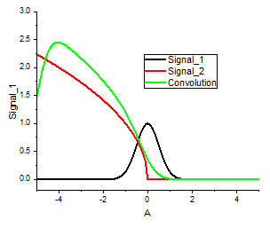
newbook s:=0 name:=Convolution;
newsheet cols:=3 xy:="XYY";
//Set up 2 signals for convolution 
Col(1)=Data(-5,10,0.1);
Col(2)=exp(-col(1)^2*2);   
Col(3)=(Col(1)<0)?sqrt(-Col(1)):0;
col(2)[L]$ = "Signal_1";
col(3)[L]$ = "Signal_2";
//calculate the convolution for signal_1 and signal_2
conv ix:=Col("Signal_1") response:=Col("Signal_2") interval:=0.1 circular:=circular oy:=<new>!(<new>,<new>);

range rr=[Convolution]2!1; // Arrange X to match original signal
rr=rr-10;
range rc=[Convolution]2!2; 
rc=rc*0.1;   //multiply convolution results by sample interval 0.1
rc[L]$="Convolution";

//plot the results in graph
plotxy (1!(1,2),1!(1,3),2!(1,2)) plot:=200;

layer.x.from=-5;
layer.x.to=5;
layer.y.from=-0.2;
layer.y.to=3;
set %C -w 1500;

Hilbert transform (Pro only)

The Labtalk Script below will introduce you how to calculate the Hilbert transform using X-function Hilbert, which gives the analytic results. Then it will plot the results into a 3D line plot with projection by using the Set and Get command.

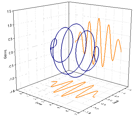
newbook sheet:=0 name:=Hilbert1;
newsheet cols:=2 xy:="XY";

//Set up data
Col(1)=Data(0,6,0.02);
Col(2)=sin(5*col(1))*sin(0.5*col(1)); 
 
//calculate the Hilbert transform;
hilbert ix:=[Hilbert1]1!2 rd:=[<input>]1!<new>;
wks.nCols = wks.nCols + 2;
wks.col6.type=6;
Col(5)=ImReal(Col(4));
Col(6)=Imaginary(Col(4));

//Set the Long name for column
col(1)[L]$ = "Time";
col(5)[L]$ = "Real";
col(6)[L]$ = "Imag";

//Plot the Hilbert transform into 3D line plot 
plotxyz iz:=(1,5,6) plot:=240;

//Set the line and symbol properties for the complex signal;
set %C -so -lo 0; // Hide droplines along Z direction
set %C -so -l 1;  // Connect symbols with Line
set %C -so -w 1500; // Set Line width
set %C -so -cl 9; // Set line color as Navy
set %C -so -z 0; // Set symbol size as 0 to hide it

set %C -sz -s 1; // Show XY projection
set %C -sz -l 1; // Connect symbols with line
set %C -sz -z 0; // Set symbol size as 0 to hide it
set %C -sz -w 1500; // Set line width
set %C -sz -cl 15; // Set line color Orange

set %C -sy -s 1; // Show XZ projection
set %C -sy -l 1; // Connect symbols with line
set %C -sy -z 0; // Set symbol size as 0 to hide it
set %C -sy -w 1500; // Set line width
set %C -sy -cl 15; // Set line color Orange

//Set the axis range
layer.x.from-=0.5;
layer.y.from-=0.5;
layer.z.from-=0.5;
layer.x.to+=0.5;
layer.y.to+=0.5;
layer.z.to+=0.5;