Curve Fitting
Contents
- 1 Linear Fit
- 2 Perform Linear Regression from a graph
- 3 Polynomial Fit
- 4 Multiple Linear Regression
- 5 Nonlinear Fit
- 5.1 Predicting Further Strengthening of the Chinese Currency
- 5.2 Fit Multiple Peaks with Replica
- 5.3 Global Fit with Parameter Sharing on Plot Segments
- 5.4 Creating Multiple Simulated Curves With a User-Defined Fitting Function
- 5.5 Fit Parameter Rearrangement in Post Fit Worsksheet Script
- 5.6 Fit Multiple Columns in a Worksheet
- 5.7 Change Parameters of an Existing Operation
Linear Fit
Fit XYYYY Data and Plot Each Fit in Separate Window
The following code will work with active book with 1st sheet having data in XYYYY form. Each Y column is fit to the first X column and a resulting fit line is added to a newly added sheet. We then plot each data and fit in a new graph.
string mybk$ = %H;  // Save the active workbook name
newsheet name:=FitLines outname:=FitLines$ cols:=1;  // Add new sheet to hold fit lines
range aa = 1!;  // 1st sheet, assume we start with just one data sheet
range bb = %(FitLines$);  // The newly added sheet, name is stored in FitLines$ variable
bb.nCols = aa.nCols;  // Add new columns in newly added sheet
// Loop all columns and perform linear fit and put results into newly added sheet
// the fitlr X-Function is used
dataset slopes, intercepts;  // To hold fitting result parameters
slopes.SetSize(aa.nCols-1);  // Number of Ys in the data worksheet
intercepts.SetSize(slopes.GetSize());  // Not needed for now, but maybe want this later
loop(ii, 2, aa.nCols) {
	range dd = 1!(1, $(ii));
	fitlr iy:=dd oy:=%(FitLines$)(1, wcol(ii));
	slopes[ii-1] = fitlr.b;  // ii-1 because loop from 2
	intercepts[ii-1] = fitlr.a;
}
// Now make a plot with all the source data and fitted data
// And add a label to show name and slope
loop(ii, 2, aa.nCols) {
	range data = [mybk$]1!(1, wcol(ii));
	range fit = %(FitLines$)(1, wcol(ii));
	win -t plot;  // Create a new graph window
	plotxy data plot:=201 ogl:=<active>;  // Plot source data as scatter
	plotxy fit plot:=200 rescale:=0 color:=color(red) ogl:=<active>;  // Plot fitted data as red line
	label -r legend;  // Don't really need a legend, delete it
	label -s -q 2 -n myLabel1 "Linear Fit to %(1, @LM)%(CRLF)slope=$(slopes[ii-1])";
}
US Total Population
The script below fit the total US population since the 1950s and project the year when the number will cross over into 400 million.
// Clean the project to start with empty space
doc -s; doc -n; {win -cd;}

// get the US population data file from SP website
string url$ = "https://fred.stlouisfed.org/data/POP";
newbook;
wbook.dc.add("HTML");
wks.dc.source$ = url$;
wks.dc.Sel$=Tables/_1;
wks.dc.import();

wks.nCols = 7;
wks.Labels(LU);
range aa = 1, bb = 2, yr = 3, pop = 4, param = 5, fitx = 6, fity = 7;
int nMonths = aa.GetSize();
yr.type = 4;  // X
yr[L]$ = "Year";
pop[L]$ = "US Population";
pop[U]$ = "Thousands";
fitx.type = 4;
fitx[L]$ = "LR Fit X";
fity[L]$ = "LR Fit Y";

int nYears = nMonths/12;  // Imported monthly data to get number of years
// Get April data to represent that year's value
for(int ii = 16, jj = 1; ii <= nMonths; ii+=12, jj++) {
	string str$ = aa[ii]$;
	string strYear$ = str.left(4)$;
	yr[jj] = %(strYear$);
	pop[jj] = bb[ii];
}
plotxy pop plot:=201 ogl:=[<new>];
y2 = 405000;  // Slightly above 400M
x2 = 2060;
fitlr;  // Fit active plot of active graph
fitx = data(x1, x2);  // Increment of 1 = 1 year
fity = fitlr.a+fitlr.b*fitx;
param[1] = fitlr.a;
param[2] = fitlr.b;
plotxy fity 200 rescale:=0 ogl:=1!;  // Use default X for fity add to layer 1 without rescale
// Add a vertical line at where the fit Y is at 400M
double yy = 400000;
double xx = (yy-fitlr.a)/fitlr.b;
type "US Population will reach 400M at year $(xx, %d)";
draw -l -v xx;
// Let also remove the legend as we don't really need it
label -r legend;
Get and Change Existing Linear Fit Operation
This example shows how to get an existing linear fit operation, then change some settings, and update the operation programmatically. This is equivalent to how user can in the GUI click the operation lock and select change parameters to change settings.
// Open sample analysis template for linear regression
string path$ = system.path.program$ + "Samples\Curve Fitting\Linear Regression.ogw";
doc -a %(path$);

// Set "Data" sheet of template active, and import sample data in one line using %@JSamples
page.active$ = "Data";
impasc fname:="%@JSamples\Curve Fitting\Sensor01.dat";

// Get the operation tree from the linear fit report sheet
op_change ir:=FitLinear1! tr:=mytree;

// Change intercept to be fixed to zero
mytree.gui.fit.FixIntercept = 1;
mytree.gui.fit.FixInterceptAt = 0;

// Set tree back to change the operation and run
op_change ir:=FitLinear1! tr:=mytree op:=run;
Apparent Linear Fit with xop X-Function and Get Result Tree
This example shows how to perform apparent linear fit by using the xop X-Function, including creating the GUI tree, setting the parameters, running the fitting and generating result tree, and printing out the result from the output result tree.
// Open sample data and create the desired graph
doc -s; doc -n; {win -cd;};  // Clean the project to start with empty space
newbook result:=apparentfit$;  // Create a new workbook for data
impasc fname:="%@JSamples\Curve Fitting\Apparent Fit.dat";  // Import sample data in one line using %@JSamples
plotxy (1,2);  // Make a scatter plot
layer.y.type = 2;  // Set Y axis type to Log10
layer -a;  // Rescale the layer

// Use the FitLinear class to create a GUI tree "lrGUI"
tree lrGUI;
xop execute:=init classname:=FitLinear iotrgui:=lrGUI;
// Use the data in the active plot, no need to set dataset
// Set Apparent Fit
lrGUI.GUI.Fit.ApparentFit = 1;
// Run the fitting and get the result into tree "lrOut"
xop execute:=run iotrgui:=lrGUI otrresult:=lrOut;
// Clean up operation objects after fit
xop execute:=cleanup;

// Get the result from the output tree and print them
type "The fitted result is:";
type "A = $(lrOut.Summary.R1.Intercept_Value), Error = $(lrOut.Summary.R1.Intercept_Error)";
type "B = $(lrOut.Summary.R1.Slope_Value), Error = $(lrOut.Summary.R1.Slope_Error)";
type "Forumla is:";
type "y = $(lrOut.Summary.R1.Slope_Value, %3.2f)x + $(lrOut.Summary.R1.Intercept_Value, %3.2f)";
Perform Linear Regression from a graph
Perform Linear Regression from a graph with multiple dataplots in a single layer. Generate all fitted lines on graph and create fitting report table.
// first import some data
filename$ = system.path.program$ + "Samples\Curve Fitting\Linear Fit.dat";
newbook;
impASC filename$;


//create a graph with the data
range data = [<active>]1!(1, 2: wcol(wks.ncols));
plotxy data plot:=201 ogl:=<active>;  // Plot source data as scatter


//use the FitLinear class to create a GUI tree "lrGUI"
tree lrGUI;
// initialize the GUI tree, with the FitLinear class
xop execute:=init classname:=FitLinear iotrgui:=lrGUI;

//Specify all data plots on graph to be input data in the GUI tree
ii = 1;
doc -e d //loop all plots in the active layer
{
	%A =  xof(%C);   //Specify XY datasets
	lrGUI.GUI.InputData.Range$(ii).X$ = %A;
	lrGUI.GUI.InputData.Range$(ii).Y$ = %C;
	range rPlot = $(ii); //define a labtalk range for each dataplot
	int uid = range2uid(rPlot); //get the uid of the range
	lrGUI.GUI.InputData.Range$(ii).SetAttribute("PlotObjUID", $(uid));  // set the uid for plot
	ii = ii + 1;
}
// perform linear fit and generate a report with the prepared GUI tree
xop execute:=report iotrgui:=lrGUI;
// clean up linear fit operation objects after fitting
xop execute:=cleanup;
Polynomial Fit
Time Series Data, Fitting the RMB Exchange Rate
When X column contains date, it is internally in Julian Days and thus some very large numbers. Internally, special code was used to shift the data so that numeric computation round-off can be minized to produce a good fit. This example shows the fit to the RMB vs USD exchange rate before year of 2010.
Following script requires the date format in your OS is MM/dd/yyyy (for example, 7/22/2005)
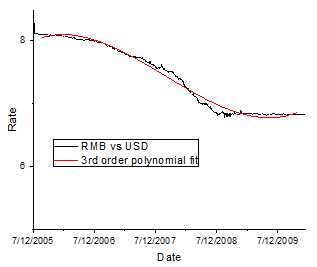
// Clean the project to start with empty space
doc -s; doc -n; {win -cd;}
newbook sheet:=1;

// Get the file from SP website
originaldcw = @DCW;
@DCW = 3; //Run Website Scripts and Direct URL

string url$ = "https://fred.stlouisfed.org/data/DEXCHUS";
wbook.dc.add("HTML");
wks.dc.source$ = url$;
wks.dc.Sel$=Tables/_1;
wks.dc.import();

@DCW = originaldcw;


wks.col1.setFormat(4, 22, yyyy'-'MM'-'dd);
range dd = 1, val = 2;
dd[C]$ = "Date"; val[C]$ = "RMB vs USD";
// Clear of the Units and Long Name imported into wrong place
dd[U]$ = ""; val[U]$ = "";
dd[L]$ = "Date"; val[L]$ = "Rate";
dd.width = 9; val.width = 7;
wks.labels(LC);

// Setup worksheet to store polynomial fit
// Setup the range variables, we are going to put all things into one worksheet
range coef = 3, fitx = 4, fity = 5, fitplot = (4, 5);
fitx = data(date(9/1/2005), date(1/1/2010), 90);
fity = fitx;  // Just to fill data so that column will be created
fitx.format = 4;  // Date
d0 = date(7/22/2005);  // X (date) to begin to range to fit
d1 = date(1/4/2010);  // X (date) to end to range to fit
ii = list(d0, col(1));  // Find corresponding row
jj = list(d1, col(1));  // Find corresponding row
// Fit 3rd order polynomial and get only coefficients
fitpoly (1, 2)[$(ii):$(jj)] 3 coef:=coef;
fity = poly(fitx, coef);

// Put in proper labels so they can appear in plot
fitx.type = 4;  // X column, not really needed for plotting, but good to see on worksheet
fity[C]$ = "3rd order polynomial fit";
plotxy (1, 2) 200;
x1 = d0-10; x2 = date(1/1/2010); x3 = 365;  // Inc by one year
y1 = 5; y2 = 8.5;
plotxy fitplot 200 rescale:=0 ogl:=1!;  // Used saved plot range and add to layer 1 without rescale
range pp = 2;  // 2nd plot is our new fit curve
set pp -c color(red);
Polynomial Fit with xop X-Function and Get Result Tree
The example below demonstrates 2nd and 3rd order polynomial fit with the xop X-Function.
// Open sample data
doc -s; doc -n; {win -cd;};  // Clean the project to start with empty space
newbook result:=polyfit$;  // Create a new workbook for data
impasc fname:="%@JSamples\Curve Fitting\Polynomial Fit.dat";  // Import sample data using one-line %@JSamples path
polyfit$ = %H;  // Get the current workbook name

// Setup the worksheet columns for the fitting results
wks.ncols = 6;  // Add 3 more columns
range coef = 4, fitx = 5, fity = 6, fitxy = (5, 6);
coef[C]$ = "coefficients of 2nd polynomial fit";
fitx.type = 4;  // X column
fitx = data(1, 100);

// Use the FitPolynomial class to create a GUI tree "polyGUI"
tree polyGUI;
xop execute:=init classname:=FitPolynomial iotrgui:=polyGUI;
// Set the input data
polyGUI.GUI.InputData.Range1.X$ = col(1);
polyGUI.GUI.InputData.Range1.Y$ = col(2);
// Run the fitting and get the result to tree "polyOut"
xop execute:=run iotrgui:=polyGUI otrresult:=polyOut;
// Clean up operation objects after fit
xop execute:=cleanup;

// Get the coefficients from the output tree
coef[1] = polyOut.Parameters.Intercept.Value;
coef[2] = polyOut.Parameters.B1.Value;
coef[3] = polyOut.Parameters.B2.Value;
// Generate the fitted Y from X
fity = poly(fitx, coef);
fity[C]$ = "2nd order polynomial fit";
// Make the plot
plotxy (1, 2);  // Scatter
plotxy fitxy 200 rescale:=0 ogl:=1!;  // Line to the same layer
range pp = 2;  // 2nd plot is the new fitted curve
set pp -c color(red);  // Set color to red

// Do the similar to column 3
win -a %(polyfit$);  // Activate the data workbook
wks.ncols = 9;  // Add 3 more columns
range coef1 = 7, fitx1 = 8, fity1 = 9, fitxy1 = (8, 9);
coef1[C]$ = "coefficients of 3rd polynomial fit";
fitx1.type = 4;  // X column
fitx1 = data(1, 100);

// Use the FitPolynomail class to create a GUI tree "polyGUI"
xop execute:=init classname:=FitPolynomial iotrgui:=polyGUI;
// Set the input data
polyGUI.GUI.InputData.Range1.X$ = col(1);
polyGUI.GUI.InputData.Range1.Y$ = col(3);
// Set order to 3
polyGUI.GUI.Order = 3;
// Run the fitting and get the result to tree "polyOut"
xop execute:=run iotrgui:=polyGUI otrresult:=polyOut;
// Clean up operation objects after fit
xop execute:=cleanup;

// Get the coefficients from the output tree
coef1[1] = polyOut.Parameters.Intercept.Value;
coef1[2] = polyOut.Parameters.B1.Value;
coef1[3] = polyOut.Parameters.B2.Value;
coef1[4] = polyOut.Parameters.B3.Value;
// Generate the fitted Y from X
fity1 = poly(fitx1, coef1);
fity1[C]$ = "3rd order polynomial fit";
// Make the plot
plotxy (1, 3);  // Scatter
plotxy fitxy1 200 rescale:=0 ogl:=1!;  // Line to the same layer
range pp1 = 2;  // 2nd plot is the new fitted curve
set pp1 -c color(red);  // Set color to red
Multiple Linear Regression
Composite Spectrum Fitting with Multiple Components
There is a data for composite spectrum (y), together with two components (x1 and x2). We assume they have the following relationship.
 Then we can perform multiple linear fit for this model by using the fitMr X-Function, so to get the related parameters of this model. That is what this example is going to show.
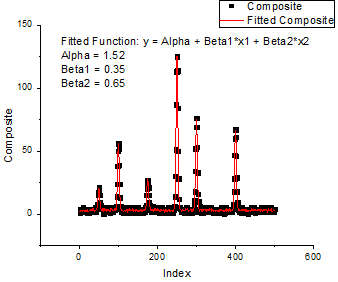
// Open sample data
doc -s; doc -n; {win -cd;};  // Clean the project to start with empty space
newbook;  // Create a new workbook for data
// Import sample data directly using %@JSamples, which maps to the Samples folder under the Origin installation
impasc fname:="%@JSamples\Curve Fitting\Composite Spectrum.dat";
wks.addCol();  // Add a column for fitted value of dependent
col(5)[L]$ = "Fitted Composite";  // Long Name

// Perform multiple linear fit
// col(4) = y, col(2) = x1, col(3) = x2, col(5) = fitted y
// Result is stored in tree trMr
fitmr dep:=col(4) indep:=col(2):col(3) mrtree:=trMr odep:=col(5);

// Plot Composite and Fitted Composite into the same graph, vs Index in col(1)
range rxy = (1, 4), rfitxy = (1, 5);
plotxy rxy 201;  // scatter
plotxy rfitxy plot:=200 rescale:=0 color:=color(red) ogl:=<active>;  // Red line plot

// Add label to show the fitting parameters
label -s -q 2 -n myLabel1 "Fitted Function: y = Alpha + Beta1*x1 + Beta2*x2
Alpha = $(trMr.v1, %3.2f)
Beta1 = $(trMR.v2, %.2f)
Beta2 = $(trMr.v3, %.2f)";
Multiple Linear Regression with xop X-Function and Get Result Tree
The expression of 3rd order polynomial fit is  . In this example, we are going to consider
  as
as  ,
,  as
as  , and
, and  as
as  , that is
  , which has 3 independents, then perform multiple linear regression with the xop X-Function, and get the result into a tree. And it will get the same parameter result as 3rd order polynomial fit.
// Open sample data
string fname$ = system.path.program$ + "Samples\Curve Fitting\Polynomial Fit.dat";
doc -s; doc -n; {win -cd;};  // Clean the project to start with empty space
newbook;  // Create a new workbook for data
impasc;  // Import data
wks.nCols = 7;  // Add 4 more columns for generating desired data
col(4) = col(1);  // X1
col(5) = col(1)^2;  // X2
col(6) = col(1)^3;  // X3
col(7) = col(3);  // Y

// Use the MR class to create a GUI tree mrGUI
tree mrGUI;
xop execute:=init classname:=MR iotrgui:=mrGUI;
// Set the input data
mrGUI.GUI.InputData.Range1.X$ = col(4):col(6);
mrGUI.GUI.InputData.Range1.Y$ = col(7);
// Run the fitting and get the result to tree mrOut
xop execute:=run iotrgui:=mrGUI otrresult:=mrOut;
// Clean up operation objects after fit
xop execute:=cleanup;

// Output the results
double alpha = mrOut.Parameters.Intercept.Value;
double beta1 = mrOut.Parameters.D.Value;
double beta2 = mrOut.Parameters.E.Value;
double beta3 = mrOut.Parameters.F.Value;
type "Alpha = $(alpha)";
type "Beta1 = $(beta1)";
type "Beta2 = $(beta2)";
type "Beta3 = $(beta3)";
type "Expression is:";
type "y = $(alpha, %4.2f) + $(beta1, %4.2f)x1 + $(beta2, %3.2f)x2 + $(beta3, %.2f)x3";
Nonlinear Fit
A new set of X-Functions to control the new Origin 8 NLFit engine were added in SR2.
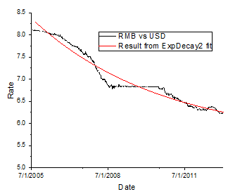
Predicting Further Strengthening of the Chinese Currency
The follow script make use of these new XF, to show how to fit the RMB and USD exchange rate since July 2005 and to extrapolate up to the year 2013. Following script requires the date format in your OS is MM/dd/yyyy (for example, 7/22/2005)
// Clean the project to start with empty space
doc -s; doc -n; {win -cd;}
newbook sheet:=1;

// Get the file from SP website
originaldcw = @DCW;
@DCW = 3; //Run Website Scripts and Direct URL

string url$ = "https://fred.stlouisfed.org/data/DEXCHUS";
wbook.dc.add("HTML");
wks.dc.source$ = url$;
wks.dc.Sel$=Tables/_1;
wks.dc.import();

@DCW = originaldcw;

wks.col1.setFormat(4, 22, yyyy'-'MM'-'dd);
range dd = 1, val = 2;
dd[C]$ = "Date"; val[C]$ = "RMB vs USD";
// Clear of the Units and Long Name imported into wrong place
dd[U]$ = ""; val[U]$ = "";
dd[L]$ = "Date"; val[L]$ = "Rate";
dd.width = 9; val.width = 7;
wks.labels(LC);

// Create a new worksheet to hold the estimates from the fitting
newsheet name:=Predict label:=Date|Estimate;
range fitx = 1, fity = 2, fitplot = (1, 2);  // Save the ranges, including fitplot for later plotting
fitx.format = 4;  // Date
fitx = data(date(9/1/2005), date(1/1/2013), 90);
fity[C]$ = "Result from ExpDecay2 fit";
page.active = 1;  // Switch back to imported data

// USD devaluation vs RMB started on July 22, 2005, ended on Jan 1, 2013
d0 = date(7/22/2005);  // Save this date
d1 = date(1/2/2013);
ii = list(d0, col(1));  // Find corresponding row
jj = list(d1, col(1));
rate0 = col(2)[ii];  // Save this value
rate1 = col(2)[jj];
plotxy (1, 2)[$(ii):$(jj)] 200;  // Plot the data since devaluation
x1 = date(7/1/2005); x2 = date(1/1/2013); y1 = 5;  // Set X, Y axis scale

// Start the fitting on the graph
nlbegin 1 ExpDecay2 tt;
tt.x0 = d0; tt.f_x0 = 1;  // First fix the x0 value at that initial date
tt.y0 = rate0; tt.f_y0 = 1;  // Also fix y0
tt.A1 = 1;
nlfit 3;  // Do only 3 iterations
tt.f_x0 = 0; tt.f_y0 = 0;  // Then relax the x0 and y0 to fit with default max iterations
nlfit;
// Now we can generate the fit curve
fity = fit(fitx);
nlend;  // All done with fitting, can terminate it now

// Add fit curve to this plot as well
// Used saved plot range and add to layer 1 without rescale
plotxy fitplot 200 rescale:=0 ogl:=1! color:=color(red);
Fit Multiple Peaks with Replica
The follow script shows how to fit a dataset, where the baselines has been subtracted, with multiple peaks.
// Clear the project to start with empty space
doc -s; doc -n; {win -cd;}

// Import sample data into a new workbook
newbook;
string fname$ = system.path.program$ + "Samples\Curve Fitting\Multiple Peaks.dat";
impAsc;

// Do fitting on col(C), we could pick any starting with col(B) in this data
range aa = (1, 3);  // A(x), C(y)
int nCumFitCol = wks.nCols+1;  // New column for the fit Y values

// For our data, we know to fit 4 gauss peaks, so set replica to 3 (peak number = replica+1)
nlbegin aa gauss tt replica:=3;
nlfit;
range yy = nCumFitCol;
yy = fit(col(1));  // Call fit(x) without peak index will generate the cummulative peak
yy[L]$ = "Fit Y";
loop(ii, 1, 4) {
	range pk = wcol(nCumFitCol+ii);
	pk = fit(col(1), ii);
	pk[L]$ = "Peak$(ii)";
}
nlend;

// Plot both src and fit in the new graph
plotxy iy:=(A,C) plot:=201 ogl:=[<new>];
plotxy iy:=[MultiplePeaks]1!(A,"Fit Y") plot:=200  ogl:=Layer1 color:=color(red);
Global Fit with Parameter Sharing on Plot Segments
The following script runs nonlinear fit to 3 exponential decay datasets on their tail segments.
doc -s; doc -n; {win -cd;}  // Clean up workspace
newbook sheet:=2;  // Data sheet and fit curve sheet
range ss2 = 2!;
ss2.name$ = "Fit Curves";
ss2.nCols = 4;  // x, fity1, 2, 3

// Switch back to first worksheet to import data
page.active = 1;
string fname$ = system.path.program$ + "Samples\Curve Fitting\Exponential Decay.dat";
impAsc;
// Save the data workbook name
string strData$ = %H;
plotxy (1, 2:end) plot:=200 ogl:=[<new>];
x1 = 0; x2 = 1.1;
sec -p 0.1;  // This is needed to allow plot to draw before we can set increment (x3)
x3 = 0.2;
sec -p 0.1;  // More time to refresh to allow subsequent range declaration to work properly
// Do fitting from 0.2 sec to the end, so need to first find the row index of 0.2 sec
range p1 = 1;  // Use first data plot, as all share same X
int i1 = xindex(0.2, p1);
range aa = (1, 2, 3)[$(i1):end];  // Select plot 1, 2, 3

nlbegin aa ExpDec1 tt;
// Share t1
tt.s_t1 = 1;
nlfit;
// Now generate the fit curves and plot them
range fx = [strData$]2!1;
fx = data(0, 1, 0.02);  // Generate the X column for all the fits
for(int ii = 1; ii <= 3; ii++) {
	range yy = [strData$]2!wcol(ii+1);
	yy[C]$ = "Fit Curve $(ii)";
	yy = fit(fx, ii);
	plotxy yy 200, ogl:=1! rescale:=0 color:=color(red);
}
nlend;
Creating Multiple Simulated Curves With a User-Defined Fitting Function
This example shows how to use nlfit X-functions to perform simulation of a user-defined fitting function. The fitting function MyFitFunc is assumed to have two parameters named a and b.
// Start a new workbook which will have two columns by default
newbook;

// Fill first column with desired X values for simulation
col(1) = {0:0.1:4};

// Leave column 2 blank and initiate fit using your function
nlbegin iy:=2 func:=MyFitFunc nltree:=mytree;

// Loop over desired parameter values, change as needed
// Here it is assumed the fitting function has two parameters: a and b
for(double a = 1.0; a < 3.0; a+=0.5) {
	for(double b = 3.0; b < 12.0; b+=2.0) {
		type "a = $(a), b = $(b)";
		// Add a new column to receive the simulated curve
		wks.addCol();
		int nCol = wks.nCols;
		// Set parameter values to tree
		mytree.a = a;
		mytree.b = b;
		// Do zero iterations to update fit
		nlfit(0);
		// Use fit() function to generate fit curve to last column using 1st column as X
		wcol(nCol) = fit(col(1));
		// Add comment to column with parameter values used
		string str$ = "a = $(a), b = $(b)";
		wcol(nCol)[C]$ = str$;
	}
}
// End the fitting process
nlend();

// Delete 2nd column which is empty, was dummy y, and then plot all columns
delete wcol(2);
plotxy (1, 2:end) 200;
To learn more about how to create a user-defined fitting function, please refer to the curve fitting tutorial
Fit Parameter Rearrangement in Post Fit Worsksheet Script
After a fit is performed, a general report sheet is created that include many output tables, among them a fitting parameters table. The layout of these tables may not be in the form that you would like them to be in, so you may need to rearrange the fit parameters and to have this rearrangement to take place automatically after the fit is recalculated.
The following example shows how you can write script to rearrange the parameters into a new sheet such that each row is for one set of data, with columns arranged as follows:
- Name, the input dataset's long name
- P1, the first parameter's value
- E1, the first parameter's error
- P2, the second parameter's value
- E2, the second paremeter's error
and so on. It will also put the reduced chisqr value into the last column.
Worksheet Script
The script should be put into the Worksheet Script dialog and have it run after the Analysis Report sheet is changed.
Tree tt;
getnlr tr:=tt iw:=__Report$ p:=1;

int nTotalParamsPerSet = 0;
for(int idx = 1; idx > 0; idx++) {
	if(tt.p$(idx) != 0/0)
		nTotalParamsPerSet++;
	else
		break;
}
nTotalParamsPerSet /= tt.nsets;

wks.nCols = 0;  // Clear the worksheet
col(1)[L]$ = "Data";
wks.col1.type = 4;  // X column

for(int nn = 1; nn <= nTotalParamsPerSet; nn++) {
	int nCol = (nn-1)*2+2;
	wcol(nCol)[L]$ = tt.n$(nn)$;
	wcol(nCol+1)[L]$ = tt.n$(nn)$ + "_Error";
	wks.col$(nCol).type = 1;  // Y column
	wks.col$(nCol+1).type = 3;  // Y Error
}

int nChiSqrCol = nTotalParamsPerSet*2+2;
wcol(nChiSqrCol)[L]$ = "Reduced Chi-Sqr";

for(int ii = 1; ii <= tt.nsets; ii++) {
	col(1)[ii]$ = tt.Data$(ii).Name$;
	for(int jj = 1; jj <= nTotalParamsPerSet; jj++) {
		int nCol = (jj-1)*2+2;
		wcol(nCol)[ii] = tt.p$((ii-1)*nTotalParamsPerSet+jj);
		wcol(nCol+1)[ii] = tt.e$((ii-1)*nTotalParamsPerSet+jj);
	}
	if(tt.nsets == 1)
		wcol(nChiSqrCol)[ii] = tt.chisqr;
	else
		wcol(nChiSqrCol)[ii] = tt.chisqr$(ii);
}
Setting up the Analysis Template
To set up the analysis template with this script, you need to do the following:
- Perform the fit as you normally would, accepting default to put report sheets into same book as the input data sheet. You should see a report sheet called FitNL1 created if you have not performed other fits in the same book, as otherwise it might be called FitNL2.
- Add a new sheet and give it any name, for example, you can call it FitParams
- With this FitParams sheet active, open from the main menu Worksheet->Worksheet Script dialog
- Copy paste the script above into the big edit box in the lower part of the dialog.
- Make sure Support Single line statements without ";" termination is unchecked, as this was due to historical reason when we allow user to enter scripts without ; termination
- Check the box Upon Changes in Range
- Enter the range string for the report sheet as FitNL1!, please note that terminating ! is needed to indicate a sheet range such that any change in that sheet will trigger this script to run.
- click the Update button to save the script to the FitParams sheet
Now if you put in new data in the original input sheet, the FitParams sheet will update to have the rearranged parameters. To then save this book as Analysis Template:
- Do a Clear Worksheet on the FitParams sheet so you know the current result is deleted.
- Click the input data sheet and also do a Clear Worksheet to ensure both the input and the report sheets are all cleaned up.
- With the input data sheet active, choose File->Save Window As from the main menu to save into an ogw file.
Now the Analysis Template is saved and you can easily open it again from File->Recent Books.
Fit Multiple Columns in a Worksheet
The following script fits multiple columns in a single worksheet and generates a table of results in a second sheet. This script requires Origin 8.1 due to the use of Function feature.
// Define a function to be used later in the script
function int FitOneData(range xyin, string strFunc$, ref tree trResults) {
	nlbegin iy:=xyin func:=strFunc$ nltree:=trResults;
	nlfit;
	nlend;
	return trResults.niter;
}

// Import sample data into new worksheet and make it active
newbook;  // Newbook default to create one worksheet
range rngSrcWks = 1!;  // Use 1st worksheet as source data
string fname$ = system.path.program$ + "Samples\Curve Fitting\Multiple Gaussians.dat";
impAsc;

// Multiple Gaussians.dat does not have column name, we will generate some
int ii;
loop(ii, 2, rngSrcWks.nCols) {
	range cc = wcol(ii);
	cc[L]$ = "Sample $(ii-1)";
}
// Create a result sheet to collect the fit result
// Only to get center and AdjR etc.
newsheet name:="Results" labels:="Name|Center|AdjR|Iterations" active:=0;
range rName = Results!col(Name);
range rCenter = Results!col(Center);
range rAdjR = Results!col(AdjR);
range rIter = Results!col(Iterations);
loop(ii, 2, rngSrcWks.nCols) {
	int rr = ii-1;
	range rngInput = (1, $(ii));
	tree tr;
	int nn = FitOneData(rngInput, "gauss", tr);
	// Put result to worksheet
	rName[rr]$ = rngInput[L]$;
	rCenter[rr] = tr.xc;
	rAdjR[rr] = tr.adjr;
	rIter[rr] = nn;
}
Change Parameters of an Existing Operation
If you have an Analysis Template and you want to change some parameter within the stored operation object, you can do that with the op_change X-Function which allows you to get and set the tree stored in the object.
// Load analysis template
string path$ = system.path.program$ + "Samples\Curve Fitting\Single Peak Fit.ogw";
doc -a %(path$);

// Partial import of data
string fname$ = system.path.program$ + "Samples\Curve Fitting\Gaussian.dat";
impAsc 	options.partImp.partial:=1
		options.partImp.firstCol:=1
		options.partImp.lastCol:=2
		orng:=Data!;

// Get the opeation tree
op_change ir:=FitNL1! tr:=tr;

// Set y0 as fixed at zero
tr.FitWorkArea.Parameters.Fixed[1] = 1;
tr.FitWorkArea.Parameters.Values[1] = 0;

// Set xc as fixed and rounded to nearest integer
tr.FitWorkArea.Parameters.Fixed[2] = 1;
tr.FitWorkArea.Parameters.Values[2] = nint(tr.FitWorkArea.Parameters.Values[2]);

// Add Fixed column to Parameters table
tr.GUI.Quantities.Parameters.Fix = 1;

// Include R value in Statistics table
tr.GUI.Quantities.Statistics.Rvalue = 1;

// Remove the ANOVA table
tr.GUI.Quantities.ANOVAtable = 0;

// Put the tree back and run the update
op_change ir:=FitNL1! tr:=tr op:=run;