2.5.11.1 Tutorial for Parametric Distribution Analysis (Arbitrary Censoring)

In this example, a company collected the battery lifetime data from periodic inspection. Engineers will now use Weibull Parametric Distribution Analysis to obtain the survival probabilities across the entire time domain, providing the quantitative basis for future decisions including warranty policy, preventive maintenance intervals, and spare-parts planning..

Topics for Parametric Distribution Analysis for Arbitrary Censoring: Algorithm

Sample Data

Right click on the Reliability and Survival app icon in the App Gallery and choose Show Sample Folder to open the sample project RSASample.opju. Go to sub-folder 2.1 Parametric Distribution Analysis (Arbitrary Censoring) .

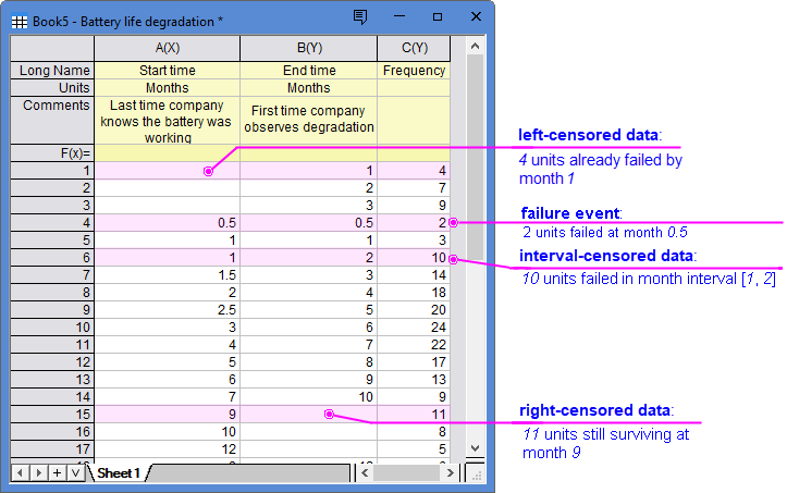
[Book5]Sheet1 shows typical arbitrary censored data - a combination of left-, right-, and interval-censored observations.

Origin’s arbitrary censoring analysis requires the censored data to be arranged in the following format:

• Start time: last time a unit was observed to be working.
• End time: first time that unit was observed failure.
  If Start time = End time, the unit faied at that exact time.
• Frequencies: count of units falling into this interval or time point.
• For left-censored units (1st to 3rd rows in this example), the "Start Time" is missing. The "Frequency" counts units already failed by the "End Time".
• For right-censored units (15th and 16th rows), the "End Time" is missing. The "Frequency" counts units still running as of the "Start Time".

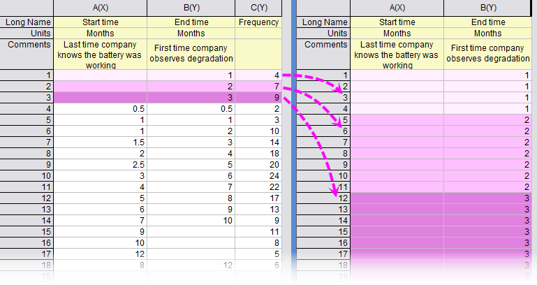
The Frequencies column is optional. If omitted, you can duplicate the interval ("Start Time" & "End Time") and each duplicate represents one failure.

Note: If your data contain only exact failure times or right-censored observations, please use Parametric Distribution Analysis for Right Censoring instead.

Steps

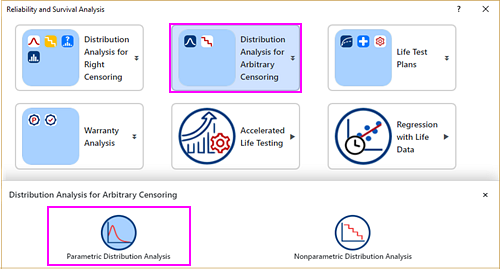
1. With [Book5]Sheet1 active, select menu Statistics: Survival Analysis: Reliability and Survival Analysis. In the opened panel, click Distribution Analysis for Arbitrary Censoring block and then choose Parametric Distribution Analysis icon.

   

2. In the dialog that opens, specify the settings as follow:
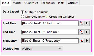
   • On the Input tab, select column A for Start Time, column B for End Time, and column C for Frequency, respectively. Choose Weibull for Distribution.

     

     Data Layout	How your data are organized. If your data contains multiple groups (e.g., different types or conditions): Multiple Columns: each group has its separate Start Time & End Time column pair; One Column with Grouping Variables: all groups are stacked in one pair of Start Time & End Time columns, with a separate grouping column. The tool will process each group in sequence, and export all results in a single report.
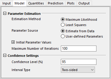
     Frequency	Optional depending on your data arrangement. Refer to "Sample Data" section for "repeating rows" vs. "frequency column".
     Distribution	Up to 7 distributions are available. Refer to this page for details of the distributions.

   • On the Model tab, Estimation Method uses Maximum Likelihood by default. Keep these settings unchanged.

     

     Estimation Method

     The algorithm used to calculate the parameters (e.g., Shape and Scale for Weibull) from your data. Refer to this page for more information about the two methods. Maximum Likelihood (MLE): recommended for moderate to large samples (>30), or data with heavy censoring. You can specify Initial Parameter Values and Maximum Number of Iterations, and export confidence band. Least Squares (Rank Regression): more stable for very small samples (<15). You can Fix Value for some parameters.

     Parameter Source

     Specify how to determine distribution parameters. Estimate from Data: use the chosen Estimation Method to calculate parameters. User-defined Parameters: use the specified User-defined Parameter Values (e.g., historical values or industry standards). No interations is performed.

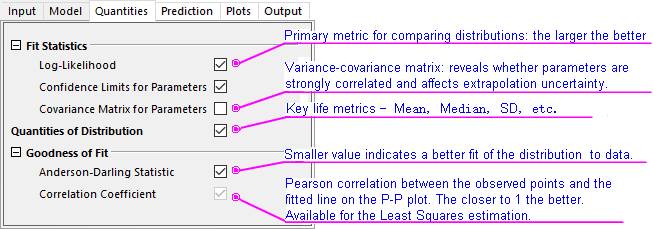
   • The Quantities tab controls which auxiliary statistics are exported besides the fitted parameters, which are essential for model validation and reliability diagnostics. Refer to "Results and Interpretation" section to see how these statistics work together to evaluate your chosen distribution model.

     

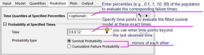
   • On the Prediction tab, you can query survival probabilities and quantiles even beyond the last observed time. Enter "3 6 9 12" (separated by space) in Time edit box to output the survival probabilities after these months elapse.

     

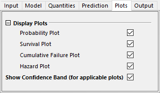
   • On Plots tab, determine which plots are output with the confidence band (if applicable). Select all by default. Refer to "Results and Interpretation" section for details of the plots.

     

3. Click OK button to generate report sheets.

Results and Interpretation

Parameter Estimates and Goodness of Fit

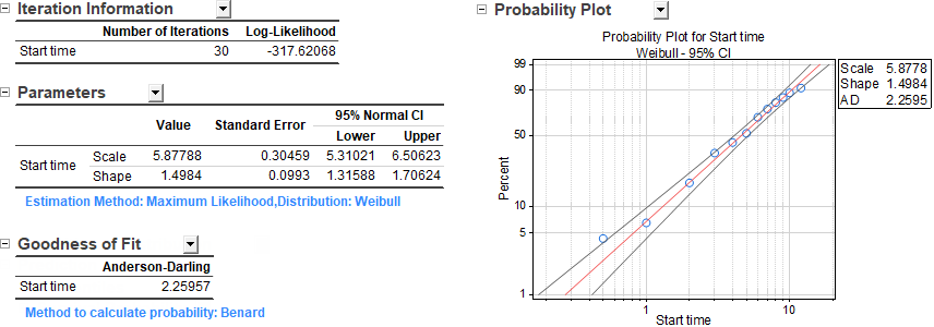
• Always validate your chosen distribution model before moving on to post-analysis such as parameter estimates and prediction.
• The Anderson-Darling and Log-Likelihood statistics alone cannot be a decisive indicator of a good model or not. You will need to diagnose in conjunction with the Probability Plot.
• The data points in the Probability Plot lie close to the Weibull theoretical line without systematic S-shaped curvature or tail deviation, and the 95% confidence band comfortably envelopes the points. The plot provides a visual inspection supporting the Weibull assumption for this heavily interval-censored dataset.
• The Parameters table provides the fitted parameters of this Weibull model with tight confidence intervals. The lower confidence bound of Shape parameter (1.316) lies well above 1.0, providing strong evidence of a classic wear-out failure mode.

Quantities of Distribution

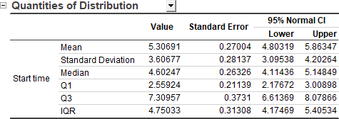
• This table reports theoretical descriptive statistics derived from the fitted Weibull distribution.
• Mean (5.31) > Median (4.60) indicates the distribution is right-skewed, a characteristic consequence of the Weibull Shape parameter ≈ 1.5. The typical lifetime of the battery is approximately 4.6 months. Roughly half of the population fails between Q1 (2.56 months) and Q3 (7.31 months). The first quartile Q1 tells that about 25% of the population will fail before 3 months, a reference for warranty planning.

Reliability Predictions

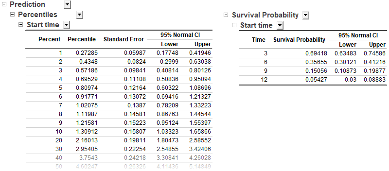
This section presents the principal predictive output of parametric analysis. Whereas nonparametric estimates are strictly bounded by the observed data range, the fitted parametric distribution enables extrapolation across the entire time domain, yielding survival probabilities and critical life percentiles.

• The Percentiles table reports Time-to-Failure quantiles. It provides the quantitative foundation for engineering decisions, such as B10 (10%) - the warranty-policy anchor point, and B50 (50%) - the Median design life. Note that the confidence bands widen with time, reflecting that the extrapolation uncertainty grows dramatically at extreme percentiles.
• The Survival Probability table reports survival probability at specified times.

Survival Plot & Cumulative Failure Plot

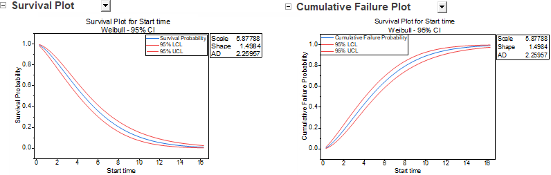
• Survival Plot and Cumulative Failure Plot provide a visual representation of the Percentiles table.

Hazard Plot

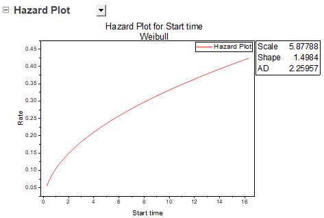
The hazard plot monotonically increases with time, indicating a classic wear-out (aging) failure mode. This is fully consistent with the Shape parameter ≈ 1.50 > 1 from the Parameters table, reinforcing the validity of the Weibull model choice.

• Early life (0 - 2 months): Hazard rate begins near 0.05; the product is relatively safe.
• Mid-life (2 – 8 months): Hazard rate climbs steadily as material degradation progresses.
• Late life (8 – 16 months): Hazard rate accelerates sharply, approaching 0.42 by month 16, indicating very high instantaneous failure risk for the few remaining survivors.