2.5.4.1 Tutorial for Identify Distribution (Right Censoring)

Indentify Distributjion creates probability plots for up to 7 distributions simultaneously, allowing you to visually compare which distribution fits your data best. The tool is used when you have incomplete observations - some units failed during testing while others were still available when data collection ended (right-censored).

In this example, a battery factory collected the battery lifetime from after-sales service data, defining lifetime as the elapsed time until capacity drops below 70 % (i.e., a 30 % loss). Engineers need to decide which distribution is the best before running post-precessing such as Parametric Distribution Analysis.

Sample Data

Right click on the Reliability and Survival app icon and choose Show Sample Folder to open the sample project RSASample.opju. Go to sub-folder 1. Distribution Analysis (Right Censoring).

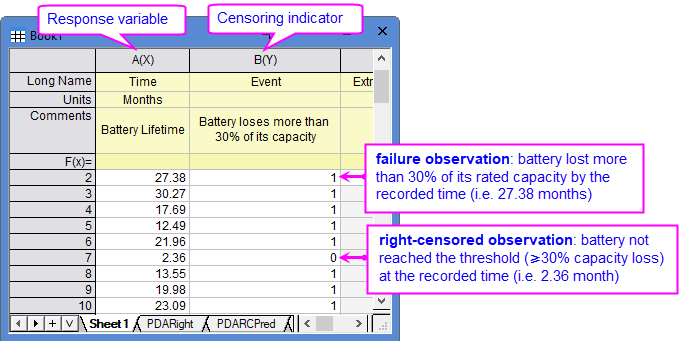
[Book1]Sheet1 shows a typical right-censored dataset.

• Each row represents one unit.
• "Time " column contains the exact failure time or the last recorded time if the unit is still working.
• "Event " column contains the censoring values: in this example, 0 = right-censored (unit still working at the record time); 1 = failure.

Steps

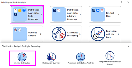
1. With [Book1]Sheet1 active, select Statistics: Survival Analysis: Reliability and Survival Analysis. In the opened panel, choose Distribution Analysis for Right Censoring block and click Identify Distribution icon.

   

2. In the dialog that opens, specify the settings as follow:
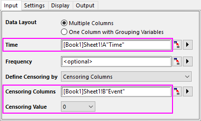
   • On Input tab, select column A for Time. Make sure Define Censoring by is set to Censoring Columns. Select column B for Censoring Columns and 0 for Censoring Value, which means any row where Event = 0 represents a unit that was still functioning at the observed time.

     

     Data Layout	How your data are organized. If your data contains multiple groups (e.g., different types or conditions): Multiple Columns: each group has its separate time & censoring column pair; One Column with Grouping Variables: all groups are stacked in one pair of time & censoring columns, with a separate grouping column. The tool will process each group in sequence, and export all results in a single report.
     Time	The column containing the observed lifetimes.
     Frequency (Optional)	When multiple units share the same observed time, you can streamline data entry by providing a frequency column rather than repeating rows. Refer to this page for "repeating rows" vs. "frequency column".
     Define Censoring by	How to distinguish failure from right-censored observations. Censoring Columns: an explicit indicator column flagging the status of each observation. The Censoring Value identifies which code means "still running". All other codes are treated as exact failure events. Time when censoring begins (Type I): units in Time column that equal or exceed the Time Value is treated as censored at exactly that time. Number of failures when censoring begins (Type II): monitoring continues until the Number of Failures have been observed. The rest are censored at that point.

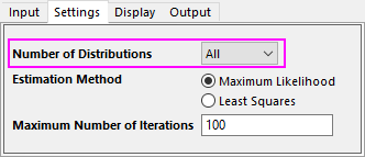
   • On Settings tab, choose All for Number of Distribution. Estimation Method defaults to Maximum Likelihood. Leave all other settings unchanged.

     

     Number of Distributions

     Choose the distributions to compare simultaneously. Choose All to compare up to 7 distributions: Normal, Lognormal, Exponential, Smallest Extreme Value, Weibull, Logistic, Loglogistic. Refer to this page for information about 7 distributions

     Estimation Method

     Choose the algorithm used to calculate the parameters (e.g., shape and scale for Weibull, location and scale for Normal) from your data. Refer to this page for algorithm of 2 methods. Maximum Likelihood (MLE): recommended for moderate to large samples (>30), or data with heavy censoring. Maximum Number of Iterations determine how many times the algorithm will attempt for parameter value optimization. Least Squares (Rank Regression): more stable for very small samples (<15). Does not require iterative optimization

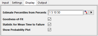
   • On Display tab, determine which results are output alongside the probability plots. Leave it as default.

     

     Refer to "Results and Interpretation" section to see how these options work together to help you evaluate and compare candidate distributions.
   • Click OK button to generate report sheets.

   Results and Interpretation

   Goodness of Fit

   

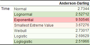
   • The Anderson-Darling statistic quantifies the discrepancy between the empirical cumulative distirbution and the fitted theoretical distribution. Smaller value indicates better fit.
   • The Exponential distribution is strongly rejected. The Loglogistic and Lognormal models yield the lowest AD; however, the difference is too small to declare a statistically meaningful advantage. The Weibull, Normal, and Logistic distributions also produce acceptable fits. The SEV model occupies an intermediate position, suggesting less representative of the underlying failure mechanism.

   
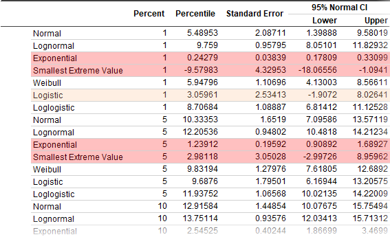
   Table of Percentiales

   

   • The percentile life estimates provide the time at which a specified cumulative percentage (st, 5th, 10th, and 50th) of the population is expected to fail. These values are particularly sensitive to distributional assumptions in the tails and often serve as the tie-breaker when AD statistics are nearly identical.
   • Candidated distributions diverge in the early-life predictions but converge to a median life of approximately 21-23 months. This consensus confirms that the choice of distribution primarily affects tail predictions (e.g., warranty forecasting)
   • The SEV model is rejected due to a negative lifetime estimate at 1st Percentile. The Exponential model is also rejected due to the near-zero estimate which is physically meaningless for a lifetime value. While the Logistic model’s 95% CI crosses 0, indicating this model is instable in the tail.

   
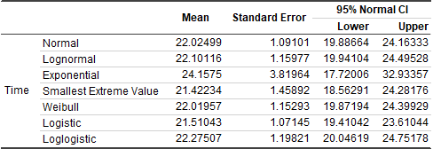
   Statistics for Mean Time to Failure

   

   • The Mean Time-to-Failure (MTTF) estimates with 95% Confidence Intervals provide a check on the central location of each distribution.
   • All candidates except Exponential produce MTTF estimates clustered around 22 months, though the SEV model shows modestly weaker performance.

   
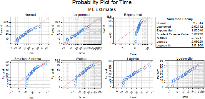
   Probability Plot

   

   • The probability plots provide the primary visual diagnostic. Under a correct model, the points should scatter randomly about the reference line without systematic curvature.
   • Exponential displays pronounced curvature, confirming the quantitative rejection by the AD statistic. SEV also shows systematic deviation in the upper tail.
   • The remaining 5 distributions (Loglogistic, Lognormal, Weibull, Logistic, Normal) all produce broadly linear patterns.

   
   Conclusion

   Both Loglogistic and Lognormal are the leading candidates based on the statstistical assessments in the report. If institutional preference or engineering judgment is considered, Weibull is the pragmatic choice given its acceptablel performance, superior physical interpretability and broader industry adoption.