2.5.8.1 Tutorial for Distribution Overview (Right Censoring)
Distribution Overview takes your chosen model and draws its complete graphical profile, and you can confirm that the fit makes physical sense before moving on to formal prediction.
Engineers in a battery factory used Identify Distribution to scan 7 candidate distributions on the collected battery lifetime data, and arrived at a conclusion that while Loglogistic and Lognormal achieved the smallest Anderson-Darling values, Weibull also produced an acceptable fit with an AD value within the same competitive cluster. Considering reliability and industry adoption, engneers prefer Weibull for the post-precessing such as Parametric Distribution Analysis.
In this example, engneers choose Weibull distribution and perform Distribution Overview to closely validate the model visually and physically across the full time domain.
Sample Data
Right click on the Reliability and Survival app icon  and choose Show Sample Folder to open the sample project RSASample.opju. Go to sub-folder 1. Distribution Analysis (Right Censoring).
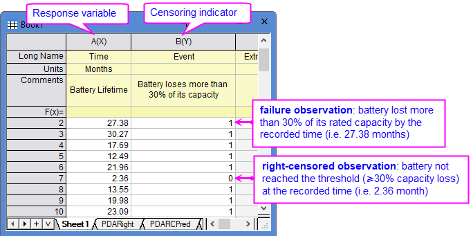
[Book1]Sheet1 shows a typical right-censored dataset.
- Each row represents one unit.
- "Time " column contains the exact failure time or the last recorded time if the unit is still working.
- "Event " column contains the censoring values: in this example, 1 = failure (battery capacity drops below 70%); 0 = right-censored (battery still working at the record time).
Steps
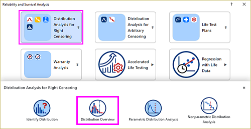
- With [Book1]Sheet1 active, select Statistics: Survival Analysis: Reliability and Survival Analysis. In the opened panel, choose Distribution Analysis for Right Censoring block and click Distribution Overview icon.
- In the dialog that opens, specify the settings as follows:
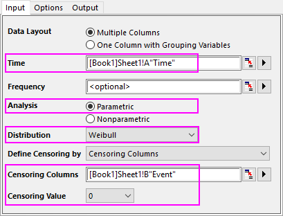
- On the Input tab, select column A for Time. Make sure Paramatric Analysis is selected and choose Weibull Distribution because Identify Distribution has already validated Weibull as an acceptable model. Select column B for Censoring Columns and 0 for Censoring Value.
Data Layout How your data are organized. If your data contains multiple groups (e.g., different types or conditions): - Multiple Columns: each group has its separate time & censoring column pair;
- One Column with Grouping Variables: all groups are stacked in one pair of time & censoring columns, with a separate grouping column.
The tool will process each group in sequence, and export all results in a single report.
Time The column containing the observed lifetimes. Frequency (Optional) When multiple units fail at the same observed time, you can streamline data entry by providing a frequency column rather than repeating rows. Refer to this page for "repeating rows" vs. "frequency column". Parametric Analysis
vs.
Nonparametric Analysis- Parametric: select an identified Distribution to see its fitted curves and estimated parameters.
- Nonparametric: makes no distributional assumption. Survival probabilities are estimated directly from the data.
Define Censoring by How to distinguish failure from right-censored observations. - Censoring Columns: an explicit indicator column flagging the status of each observation. The Censoring Value identifies which code means "still running". All other codes are treated as exact failure events.
- Time when censoring begins (Type I): units in Time column that equal or exceed the Time Value is treated as censored at exactly that time.
- Number of failures when censoring begins (Type II): monitoring continues until the Number of Failures have been observed. The rest are censored at that point.
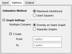
- On the Options tab, make sure Maximum Likelihood is selected for Estimation Method. Leave other settings unchanged.
Estimation Method - When Parametric anallysis is selected on the Input tab, choose the algorithm used to calculate the parameters (e.g., shape and scale for Weibull, location and scale for Normal) from your data. Refer to this page for algorithm of 2 methods.
- Maximum Likelihood (MLE): recommended for moderate to large samples (>30), or data with heavy censoring.
- Least Squares (Rank Regression): more stable for very small samples (<15).
- When Nonparametric analysis is selected on the Input tab,
- Kaplan-Meier: Computes survival probability at each exact failure time. Recommended when you have precise failure times and want the most detailed, step-by-step survival curve.
- Actuarial: Groups data into time intervals by Interval End and Interval Width, and computes survival probability at each interval boundary. Recommended when your data are already grouped, or when you have so many data that a step-for-step KM curve becomes unreadable.
Graph Settings - Multiple Columns: If your data contains multiple time&event pairs, you can choose whether to plot all pairs Overlay on Same Graph, or in Separate Graphs.
- X Scale: If you want to inspect a specific time window closely, e.g., early-life behavior, set From and To to zoom in on that time interval for all output plots.
Note: this setting does not change the underlying calculation; it only adjusts the graph display.
- Click OK button to generate report sheets.
Results and Interpretation
Parameters
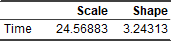
- This table lists the fitted parameters of Weibull distribution. Shape parameter 3.24 > 1 indicates a wear-out failure mechanism, i.e., the longer a battery runs, the higher its instantaneous risk of failure.
Quantities of Distribution- This table lists the key Times of survival rates. Roughly half of the population fails between Q1 (16.73 months) and Q3 (27.17 months). The first quartile Q1 (16.73 months) tells us that about 25% of the population will fail before 17 months.
- The Mean (22.02 months) and Median (21.94 months) are nearly identical. This near-symmetry is consistent with the Shape parameter of 3.24 (reported in the Parameters table), approaching the near-symmetric region (Shape ≈ 3.4 – 3.6) of the Weibull distribution.
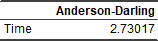
Goodness of Fit- This table reports an acceptable Anderson-Darling statistic (2.73) of the Weibull distribution. This value is consistent with the result from Identify Distribution.
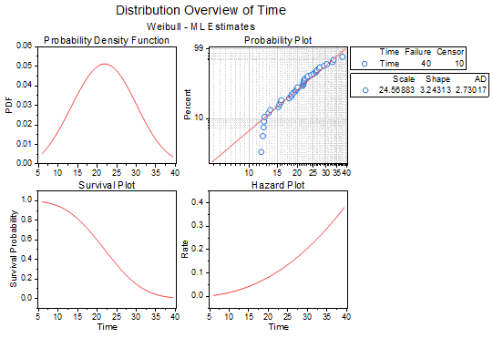
Distribution Overview Graphs- Probability Density Function: A single, well-defined peak centered near 22–24 months with a moderate right tail, consistent with a wear-out process.
- Probability Plot: The points scatter randomly around the reference line without systematic curvature, validating the Weibull assumption.
- Survival Plot: The curve falls smoothly from 1.0. At 20 months, about 50% batteries are still working; by 30 months, only 10% remain.
- Hazard Plot: The curve rises monotonically from near-zero to over 0.35, confirming that failure risk accelerates with age.
Conclusion- Taken together, all plots and the parameter estimates tell the same physically sensible story: battery capacity degrades through a wear-out process with a characteristic life near 25 months. The model is stable, the fit is acceptable, and the Weibull assumption is ready for Parametric Distribution Analysis.
- On the Input tab, select column A for Time. Make sure Paramatric Analysis is selected and choose Weibull Distribution because Identify Distribution has already validated Weibull as an acceptable model. Select column B for Censoring Columns and 0 for Censoring Value.