2.5.2.1 Tutorial: Non-Parametric Distribution Analysis (Right Censoring)

Nonparametric analysis estimates the survival function without any parametric distribution assumption. Therefore, it offers an unbiased, data-driven description of survival probabilities and serves as a robust tool for summarizing right-censored data and diagnosing which parametric models are visually and numerically validated.

Topics for Nonparametric Distribution Analysis for Right Censoring: Algorithm

In this example, engneers in a battery factory will perform Nonparametric Distribution Analysis on the collected battery lifetime data to draw the depiction of survival probabilities across the observed time interval.

Sample Data

Right click on the Reliability and Survival app icon and choose Show Sample Folder to open the sample project RSASample.opju. Go to sub-folder 1. Distribution Analysis (Right Censoring).

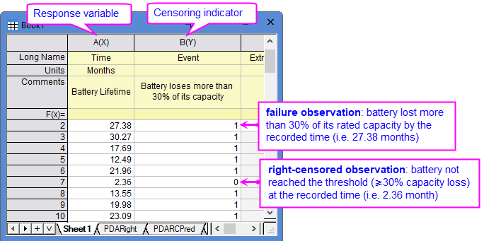
[Book1]Sheet1 shows a typical right-censored dataset.

• Each row represents one unit.
• "Time " column contains the exact failure time or the last recorded time if the unit is still working.
• "Event " column contains the censoring values: in this example, 1 = failure (battery capacity drops below 70%); 0 = right-censored (battery still working at the record time).

Steps

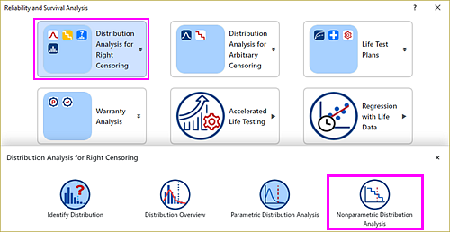
1. With [Book1]Sheet1 active, select Statistics: Survival Analysis: Reliability and Survival Analysis. In the opened panel, choose Distribution Analysis for Right Censoring block and click Nonparametric Distribution Analysis icon.

   

2. In the dialog that opens, specify the settings as follows:
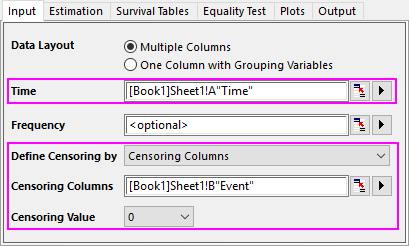
   • On the Input tab, select column A for Time. Make sure Define Censoring by is set to Censoring Columns. Select column B for Censoring Columns and 0 for Censoring Value.

     

     Data Layout	How your data are organized. If your data contains multiple groups (e.g., different types or conditions): Multiple Columns: each group has its separate time & censoring column pair; One Column with Grouping Variables: all groups are stacked in one pair of time & censoring columns, with a separate grouping column. The tool will process each group in sequence, and export all results in a single report.
     Time	The column containing the observed lifetimes.
     Frequency (Optional)	When multiple units fail at the same observed time, you can streamline data entry by providing a frequency column rather than repeating rows. Refer to this page for "repeating rows" vs. "frequency column".
     Define Censoring by	How to distinguish failure from right-censored observations. Censoring Columns: an explicit indicator column flagging the status of each observation. The Censoring Value identifies which code means "still running". All other codes are treated as exact failure events. Time when censoring begins (Type I): units in Time column that equal or exceed the Time Value is treated as censored at exactly that time. Number of failures when censoring begins (Type II): monitoring continues until the Number of Failures have been observed. The rest are censored at that point.

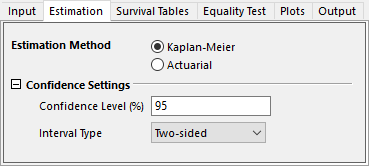
   • On the Estimation tab, make sure Kaplan-Meier is selected for Estimation Method. Leave other settings unchanged.

     

     Estimation Method

     Kaplan-Meier: Computes survival probability at each exact failure time. Recommended when you have precise failure times and want the most detailed, step-by-step survival curve. Actuarial: Divide data into time intervals by specifying a column of Endpoints of Intervals (unevenly spacing intervals are supported), and computes survival probability at each interval boundary. Recommended when your data are already binned by time intervals, or when you have so many data that a step-for-step KM curve becomes unreadable.

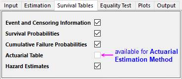
   • On the Survival Tables tab, select Event and Censoring Information, Survival Probabilities, Cumulative Failure Probabiities and Hazard Estimates checkboxes to export all of these tables. Refer to "Results and Interpretation" section for details of these tables.

     

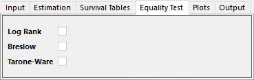
   • The Equality Test tab is available for comparing survival curves among multiple groups. This example has only one group so leave this tab untouched.

     

     Log Rank	A rank-based test that weights all event times equally when accumulating group differences. Suitable when group differences are expected to be consistent across the entire study duration, or the proportional hazards assumption is plausible. It is the defuault and most widely used test.
     Breslow	A weighted rank test that assigns greater contribution to early event times. Suitable when you suspect the strongest group separation occurs in the early period.
     Tarone-Ware	A compromise test that down-weights late events less aggressively than Breslow but still emphasizes the early-to-mid period. Suitable when you believe differences are concentrated in the early-to-middle period and you want a balanced alternative between the uniform weighting of Log Rank and the extreme early emphasis of Breslow.

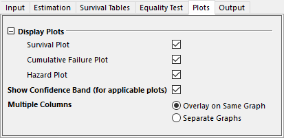
   • On the Plots tab, check to export Survival Plot, Cumulative Failure Plot, and Hazard Plot and Show Confidence Band for applicable plots. Refer to "Results and Interpretation" section for details of these plots.

     

   • Click OK button to generate report sheets.

   Results and Interpretation

   Characteristics of Variables

   

   • This table reports the descriptive statistics of the right censored data. The MTTF (21.95 months) and Median (21.69 months) are very close, indicating that the failure-time distribution is roughly symmetric. The typical lifetime of the battery is approximately 22 months.

   
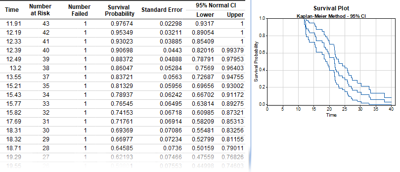
   Survival Probabilities & Survival Plot

   

   • The numeric table outputs the survival probability and its precision metrics (standard error and confidence bands) at each observed event time, from which you can tell the survival patterns: survival probability drops monotonically from 0.977 at 11.91 months to 0.029 at 37.73 months.
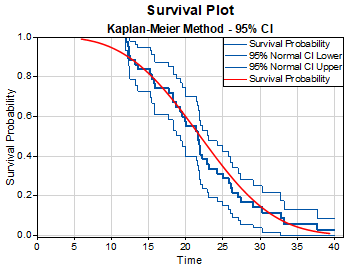
   • This pattern also visualizes in the Survival Plot: the Kaplan–Meier curve descends stepwise from approximately 100% before 10 months to near 0% after 37 months.
   • The Survival Probabilities and Cumulative Failure Probabilities are mirrors of each other, so exporting the Survival Probabilities table alone is sufficient for most reporting purposes. And the Survival Probabilities and Hazard Estimates together depicts the whole picture of your right censored data.

   
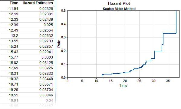
   Hazard Estimates & Hazard Plot

   

   The Hazard Estimates table is the most critical diagnostic if you want to select an appropriate parametric model in the subsequent process.

   • The hazard rate increases monotonically with time, indicating a classic wear-out failure mode: failure rate in early-life is low, but climbs continuously as aging progresses, reaching 0.5, a very high instantaneous failure intensity, by 37 months.
   • This monotonically increasing hazard is fully consistent with a Weibull distribution with Shape parameter > 1.
   • Hazard plot visually confirms the monotonically increasing hazard identified in the numeric table. Note that estimates beyond 30 months (exaggerated step) are unstable due to sparse risk sets

   
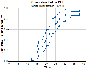
   Cumulative Failure Plot

   

   • The mirror image of the Survival Plot. It shows, for example, that roughly 40% of units have failed by 20 months and approximately 90% have failed by 30 months.

   
   Conclusion

   • The Wear-out failure mode read from hazard rate indicates that Weibull should be the primary candidate in the subsequent parametric analysis.
   • After performing a Weibull Parametric Distribution Analysis, you can overlay the fitted curve (red line shown below) on the Kaplan–Meier plot to visually validate that the model captures the observed wear-out behavior.