2.17 Probability Distribution Calculator (Pro)

Summary

The tool Critical Value of Distributions is used to calculate critical values of common distributions, such as Normal, LogNormal, t, F, Chi-squared, Hypergeometric, Geometric, Beta, Exponential, Gamma, Weibull, Uniform, Binomial and Poisson. The critical values can be (1) probability density, (2) cumulative probability, and (3) values of inverse cumulative probabliity.

Examples

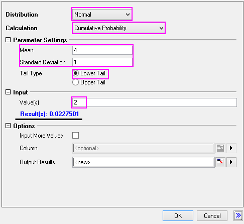
We want to calculate cumulative probability of Normal distribution at \(x=2\) with parameters mean = 4 and standard deviation = 1.

1. This is a build-in App with Origin. If you haven't this tool, you can search the Probability Distribution Calculator in App Center to install it.
2. Select Statistics: Descriptive Statistics: Probability Distribution Calculator or click the Probability Distribution Calculator app icon in App Galler to open the app dialog
3. Choose Normal for the Distribution;
4. Choose Cumulative Probability for the Calculation;
5. In the part of Parameter Settings: let Mean = 4 and Standard Deviation=1, and then choose Lower Tail for the Tail Type;
6. In the part of Input: type 2. And we get the result is 0.0227501 below.

   

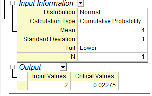
7. Click OK to get the report table.

   

Dialog Settings

Distribution

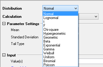
Specify which distribution to concern. Normal, LogNormal, t, F, Chi-squared, Hypergeometric, Geometric, Beta, Exponential, Gamma, Weibull, Uniform, Binomial and Poisson distributions are available now.

Calculation

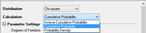
Specify which type of critical values to calculate.

1. For continuous probability distributions such as Normal, LogNormal, t, F, Chi-squared, Beta, Exponential, Gamma, Weibull and Uniform, the values of probability density, cumulative probability, and inverse cumulative probability can be calculated.
2. For discrete probability distributions such as Hypergeometric, Geometric, Binomial and Poisson, the values of probability density and cumulative probability can be calculated.

Parameter Settings

Set the values of parameters for the specific distribution chosen already.

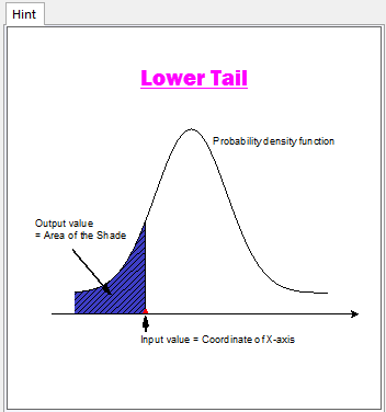
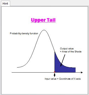
For Cumulative Probability and Inverse Cumulative Probability settings, Tail Type option is available to specify which tail type to calculate. The meaning of Lower Tail and Upper Tail is obvious by seeing the figure in the Preview window right to the setting dialog.

Input

Specify values at which the critical values of distribution are calculated. Several values can be input at the same time, separating by a space.

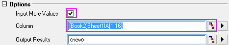
Options

Input more values from Worksheet and output the results.

Formulas

Normal distribution

The Normal distribution is also called Gaussian distribution. The probability density function is

\[f(x)=\frac{1}{\sqrt{2\pi}\sigma}e^{-\frac{(x-\mu)^2}{2\sigma^2}},\]

where \(\mu\) is the mean parameter; \(\sigma>0\) is standard deviation parameter; and \(-\infty < x < \infty\).

Lognormal distribution

The probability density function is

\[f(x)=\frac{1}{\sqrt{2\pi}\sigma(x-\theta)}e^{-\frac{(\ln(x-\theta)-\mu)^2}{2\sigma^2}},\]

where \(\mu\) is the scale parameter; \(\sigma>0\) is location parameter; \(\theta\) is threshold parameter; and \(x > \theta\).

t distribution

The probability density function is

\[f(x)=\frac{\Gamma[(v+1)/2]}{\Gamma(v/2)\sqrt{\pi v}}\left(1+\frac{x^2}{v}\right)^{-(v+1)/2},\]

where \(v\) is degree of freedom; and \(-\infty < x < \infty\). \(\Gamma\) is the Gamma function.

F distribution

The probability density function is

\[f(x)=\frac{\Gamma[(v+u)/2]}{\Gamma(v/2)\Gamma(u/2)} \left(\frac{u}{v}\right)^{u/2} x^{\frac{u}{2}-1} \left(1+\frac{u}{v}x\right)^{-(v+u)/2},\]

where \(u>0\) is numerator degree of freedom; \(v>0\) is denominator degree of freedom; and \(x>0\).

Chi-squared distribution

The probability density function is

\[f(x)=\frac{x^{(v-2)/2}e^{-x/2}}{2^{v/2}\Gamma(v/2)},\]

where \(v>0\) is degree of freedom; and \(x>0\).

Hypergeometric distribution

The probability density function is

\[f(x)=\frac{\binom{N_1}{x}\binom{N_2}{n-x}}{\binom{N}{n}},\]

where \(N = N_1+N_2\) is population size; \(N_1\) is number of events in the population; \(N_2\) is number of nonevents in the population; \(n\) is sample size; and \(x\) is number of events in the sample, s.t. \(\max\{0,n-N_2\}<x<\min\{n,N_1\}\).

Geometric distribution

If the domain is \(\{1,2,3,\cdots\}\), then the probability density function is

\[f(x)=p(1-p)^{x-1},\]

where \(p\) is event probability; and \(x\in \{1,2,3,\cdots\}\) is the total number of trials.

If the domain is \(\{0,1,2,3,\cdots\}\), then the probability density function is

\[f(x)=p(1-p)^{x},\]

where \(p\) is event probability; and \(x\in \{0,1,2,3,\cdots\}\) is the total number of nonevents occured before the first event is observed.

Beta distribution

The probability density function is

\[f(x)=\frac{\Gamma[\alpha+\beta]}{\Gamma(\alpha)\Gamma(\beta)} x^{\alpha-1}(1-x)^{\beta-1},\]

where \(\alpha>0\) is first shape parameter; \(\beta>0\) is second shape parameter; and \(0 \leq x \leq 1 \).

Exponential distribution

The probability density function is

\[f(x)=\frac{1}{\mu}e^{-(x-\theta)/\mu},\]

where \(\mu>0\) is scale parameter; \(\theta\) is threshold parameter; and \(x >\theta \).

Gamma distribution

The probability density function is

\[f(x)=\frac{(x-\theta)^{\alpha-1}}{\Gamma(a)b^a} e^{-(x-\theta)/b},\]

where \(a>0\) is shape parameter; \(b>0\) is scale parameter; \(\theta\) is threshold parameter; and \(x >\theta \).

Weibull distribution

The probability density function is

\[f(x)=\frac{\beta (x-\theta)^{\beta-1}}{\alpha^\beta} e^{-\left(\frac{x-\theta}{\alpha}\right)^\beta},\]

where \(\alpha>0\) is scale parameter; \(\beta>0\) is shape parameter; \(\theta\) is threshold parameter; and \(x >\theta \).

Uniform distribution

The probability density function is

\[f(x)=\frac{1}{b-a},\]

where \(a\) is lower endpoint; \(b\) is upper endpoint; and \(a\leq x \leq b \).

Binomial distribution

The probability density function is

\[f(x)=\binom{n}{x}p^x(1-p)^{n-x},\]

where \(n\) is number of trials; \(p\) is event probability; and \(x \in \{0,1,2,\cdots,n\} \).

Poisson distribution

The probability density function is

\[f(x)=\frac{\theta^x}{x!}e^{-\theta},\]

where \(\theta>0\) is mean; and \(x \in \{0,1,2,\cdots\} \). link title

Smallest Extreme Value distribution

The probability density function is

\[ f(x) = \frac{1}{\beta } e^{ \frac{x- \alpha}{\beta}} e^{ - e^{ \frac{x- \alpha}{\beta} } } \; \beta>0\]

Largest Extreme Value distribution

The probability density function is

\[f(x) = \frac{1}{\beta } e^{- \frac{x- \alpha}{\beta}} e^{ - e^{ -\frac{x- \alpha}{\beta} } }, \; \beta>0\]

Logistic distribution

The probability density function is

\[f(x) = \frac{\exp\left(\frac{x-\mu}{\sigma}\right)}{\sigma\left[1+\exp\left(\frac{x-\mu}{\sigma}\right)\right]^2}, \quad -\infty < x < \infty \quad \sigma > 0\]

Log-logistic distribution

The probability density function is

\[f(x) = \frac{\exp\left(\frac{\ln x-\mu}{\sigma}\right)}{x\sigma\left[1+\exp\left(\frac{\ln x-\mu}{\sigma}\right)\right]^2}, \quad x > 0 , \sigma > 0\]

Folded Normal distribution

The probability density function is

\[ f(x)= \frac{1}{ \sqrt{ 2 \pi } \sigma} e^{ - \frac{(x - \mu)^2}{ 2 \sigma^2 } } + \frac{1}{ \sqrt{ 2 \pi } \sigma} e^{ - \frac{(x + \mu)^2}{ 2 \sigma^2 } }, \; x \geqslant 0\]

Rayleigh distribution

The probability density function is \(f(x) = \frac{x}{\sigma^2} \exp\left(-\frac{x^2}{2\sigma^2}\right), \quad x \geq 0, \quad \sigma > 0\)

Gaussian Mixture distribution

The probability density function is \(f(x) = \sum_{k=1}^{K} \pi_k \cdot \frac{1}{\sigma_k\sqrt{2\pi}} \exp\left(-\frac{(x-\mu_k)^2}{2\sigma_k^2}\right)\)