Hinweis:Dieser Abschnitt ist nur in englischer Sprache verfügbar. Wir bitten um Ihr Verständnis.
2.66 Empirical Mode Decomposition (Pro)
Summary
This Empirical Mode Decomposition app can be used to perform Empirical Mode Decomposition, and Spectrum Analysis including Frequency Transform and Hilbert-Huang transform.
The App requires Python library emd. The library and other dependent Python libraries will be automatically installed when the App is launched the time.
Tutorial
- Open a new project or a new workbook. Generate XY data with steps in section below. We will get a skewed, nonlinear near-bed wave
-
- Highlight column B, and then click the Empirical Mode Decomposition icon,
 , from Apps Gallery.
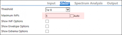
 - When the dialog is open, switch to Sifting tab, clear the checkbox of Maximum IMFs line, and then set this parameter to 5.
-
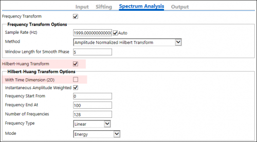
- Go to Spectrum Analysis tab, select the Hilbert-Huang Transform checkbox, and then under Hilbert-Huang Transform Options group, clear With Time Dimension (2D) checkbox.
-
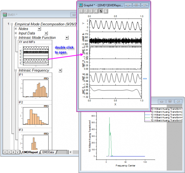
- Click Output tab, and change Output to New Book.
- Click OK.
-
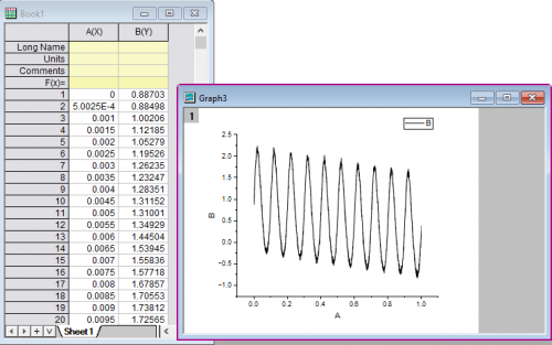
Generating data of skewed, nonlinear near-bed wave
To simulate a non-linear waveform using equation 9 in [1].
| \[u(t)=U_wf\frac{\left [sin(\omega t)-\frac{r}{1+\sqrt{1-r^2}}\right ]}{[1-rsin(\omega t)]}\] | (9) |
- Choose menu Window: Script Window to open Script Window if it is not yet open
- Copy and paste scripts below in Script Window, highlight all lines and press Enter to run them
range rx = [Book1]Sheet1!col(A);  // Column A range
range ry = [Book1]Sheet1!col(B);  // Column B range

sample_rate = 2000;  // Sampling frequency
seconds = 1;  // Number of seconds
num_samples = sample_rate * seconds;  // Number of samples
f = 10;  // Fundamental frequency
nonlin_deg = 0.25;  // Degree of non-linearity
nonlin_phi = -pi / 4;  // Skew in non-linearity

rx = data(0, seconds, seconds / (num_samples-1));  // Generate the time vector, and put it to column A

// The following is the equation 9 in [1]
factor = sqrt(1-nonlin_deg*nonlin_deg);
num = nonlin_deg * sin(nonlin_phi) / 1 + factor;
numerator = num + sin(2*pi*f*rx);
denominator = 1 - nonlin_deg * cos(2*pi*f*rx + nonlin_phi);
ry = factor * (numerator / denominator);

ry = ry  - sin(2*pi*0.1*rx);  // Add part of cycle as a trend
white_noise ry;  // Add some noise
[1] Abreu, T., Silva, P. A., Sancho, F., & Temperville, A. (2010). Analytical approximate wave form for asymmetric waves. Coastal Engineering, 57(7), 656–667. https://doi.org/10.1016/j.coastaleng.2010.02.005