2.42.5 The Overlaid Contour Plot in DOE
Contents
Introduction

The Overlaid Contour Plot lets you display contour lines for multiple responses from a designed experiment on a single graph, so you can find factor settings that satisfy all response requirements at once.
Supported design types
 | To create an overlaid contour plot, the design should include at least 2 numeric factors and 2 responses (a report must exist for each response) |
To create the overlaid contour plot
- Create the design with at least two numeric factors and 2 responses
- Analyse the design for all responses (Perform analyse design for each response one by one and create the reports)
- Select Statistics: Quality Improvement: Design of Experiment from the Origin menu
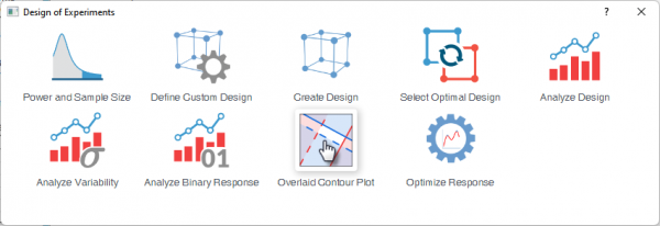
- Select the Overlaid Contour Plot icon
Understanding the Plot
An overlaid contour plot displays two or more fitted response surfaces in the same factor space—typically for two factors, with the remaining factors held constant. Each response is drawn with its own colored contour lines and bands, showing how its predicted value changes across the design region.
Origin draws a contour line at each response's Low and High acceptance limits and shades the region outside those limits. The plot is read as follows:
- Colored band (single color): the response of that color is not satisfied here - it lies outside its acceptance limits - while the other response(s) are satisfied.
- White / unshaded region: the feasible region, or "sweet spot"—every response is within its limits at once. This is the set of factor combinations that satisfies all response constraints simultaneously.
- Overlapping colored bands: all the overlapping responses are outside their limits—none is satisfied there.
In short, any shaded area means at least one response fails its requirement; only the white region meets all of them.
The Overlaid Contour Plot Dialog Box
Overlaid Contour Plot - Standard
Setup
| Responses & Limits |
|
|---|---|
| Axes |
|
| Gridding |
|

Hold Values
This controls what happens to the factors not shown on the X and Y axes. Since an overlaid contour plot can only display two factors at a time, every other factor must be "held" at a fixed value while Origin computes the predicted responses across the plot grid.
| Continuous Factors | Choose the hold value for the continuous factor from the dropdown
|
|---|---|
| Categorical Factors | The fixed level of any categorical factor |
Overlaid Contour Plot - Mixture Design
Setup
| Responses & Limits |
|
|---|---|
| Axes Mode |
|
| Component Unit |
|
| Gridding |
|
Hold Values
Set fixed (held) values for predictors not plotted on the contour axes, so the fitted model can be evaluated over the grid defined on the Setup tab.
| Components |
| |
|---|---|---|
| Process Variables |
|
|
| Mixture Amount | Enable only when model terms include total amount
Select the fixed level for mixture amount |