2.42.3.3.1 Interpreting Results for Analyze Design
Contents
Report Sheet
The tables in the section are included in the report sheet for analyze design, which is named DOEAnalysis
Coded Coefficients
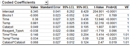
The coded coefficients table presents the regression coefficients using standardized (coded) factor levels, typically ranging from −1 to +1.
Coefficients
The estimated model coefficients (slopes) for each factor and interaction.
- Larger absolute coefficient values indicate stronger effects.
- Significant interaction coefficients indicate the effect of one factor depends on the level of another factor.
- Positive coefficient → Increasing the factor increases the response.
- Negative coefficient → Increasing the factor decreases the response.
Standard Error
The precision of each coefficient estimate. Smaller values mean more reliable estimates.
Confidence Limits (95% LCL, 95% UCL)
The lower and upper bounds of the confidence interval for each coefficient, based on the chosen confidence level.
t-Value
The test statistic used to judge whether a coefficient is significantly different from zero.
Prob>|t|
The p-value associated with the t-test. Values below your significance threshold (commonly 0.05) indicate significant terms.
VIF
Variance Inflation Factor. Values much larger than 1 suggest multicollinearity among model terms.
Example
| Term | Coefficient | Interpretation |
|---|---|---|
| A | 3.12 | Increasing factor A increases the response. |
| B | -1.75 | Increasing factor B decreases the response. |
| AB | 2.05 | Factors A and B interact significantly. |
Regression Equation in Coded Units
The coded regression equation predicts the response using standardized factor levels.
Uncoded Coefficients
The uncoded coefficients are expressed using the actual experimental units.
Example:
| Factor | Coefficient |
|---|---|
| Temperature (°C) | 0.42 |
| Pressure (bar) | -0.18 |
Regression Equation in Uncoded Units
Provides a prediction equation using actual operating conditions.
Statistics
R-Square
Represents the percentage of response variation explained by the model.
- > 0.9: Excellent
- 0.8 ~ 0.9: Good
- 0.7 ~ 0.8: Acceptable
- < 0.7: Model may require improvement
Adj. R-Square
Adjusted R-square, which accounts for the number of predictors in the model. It penalizes over-fitting and is the preferred metric when comparing models with different numbers of terms
PRESS
Predicted Residual Sum of Squares. A measure of how well the model predicts new observations, calculated by iteratively leaving out one observation at a time. Smaller is better.
Residual Sum of Square
Residual Sum of Square is actually the sum of the square of the vertical deviations from each data point to the fitting regression line. It can be inferred that your data is perfect fit if the value of RSS is equal to zero
Root-MSE (SD)
The square root of the mean square error. It estimates the standard deviation of the random error (noise) around the fitted model. Smaller is better.
Pred. R-Square
Predicted R-square. It estimates how well the model predicts future observations. A value close to the R-square indicates the model is not over-fitted and will generalize well
AIC
Akaike Information Criterion. It evaluates model fit while penalizing model complexity. When comparing models fitted to the same data, a smaller AIC generally indicates a better balance between fit and complexity.
AICc
Corrected Akaike Information Criterion. It applies an additional correction to AIC for smaller sample sizes. As with AIC, smaller values indicate a preferable model when comparing models fitted to the same data
BIC
Bayesian Information Criterion. Like AIC, BIC balances model fit and complexity, but applies a stronger penalty for additional model terms. A smaller BIC generally indicates a better model when comparing competing models.
ANOVA
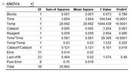
The ANOVA (Analysis of Variance) table tests whether each term contributes significantly to explaining the response.
- Chi-Sqaure/F-Value
- Higher Chi-Sqaure/F-values indicate stronger factor effects.
- Prob < ChiSq/Prob < F
- P > 0.05: Good model fit.
- P < 0.05: Model may not adequately represent the data.
Lack of Fit
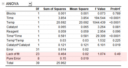
The Lack of Fit test is used to determine whether the selected model adequately describes the relationship between the factors and the response.
The test separates the model error into two components:
- Lack of Fit
- Pure Error
The Lack of Fit Test compares these two sources of variation using an F-test:
\[ F = \frac{\text{Mean Square of Lack of Fit}}{\text{Mean Square of Pure Error}} \]
The test results are in the ANOVA table of report sheet.
Lack of Fit
Variation indicating that the model does not adequately capture the true relationship between the factors and the response
A small p-value indicates significant lack of fit
- P > 0.05: The model fits the data adequately
- P < 0.05: Indicates significant lack of fit, suggesting that the model may be inadequate and that a different model or additional terms may be needed.
Pure Error
Variation caused by random experimental error, estimated from replicated experimental runs.
Means Table
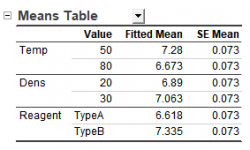
The means table shows the average response at each factor level.
Response Table
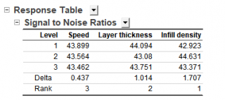
The response tables, available for Taguchi Design, summarizes how each control factor affects the response at its different levels. It helps identify the optimal factor levels and rank the relative importance of the factors.
| Signal to Noise Ratios (S/N) | The S/N ratio combines the mean response and variation into a single metric. A higher S/N ratio indicates a more robust setting (better quality with less sensitivity to noise). |
|---|---|
| Means/Slope |
|
| Standard Deviations | The table shows shows the average standard deviation of the response at each factor level. It helps identify which factor settings reduce process variation. |
The tables include following results
- Level
- The setting of a factor (here, three levels per factor).
- Delta
- The difference between the maximum and minimum level average for that factor. A larger Delta means greater influence.
- Rank
- The relative importance ordering (1 = most important, 3 = least important).
Diagnostics
The diagnostics are displayed in fitted result worksheet, named DOEFittedResult
Standard DOE Diagnotics/Fitted Results
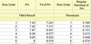
The worksheet presents the fitted results from the standard factorial/RSM analysis
Observation
Observed response values from the experiment.
Fitted Values
Values predicted by the fitted model for each run.
Regular Residuals
The regular residuals also called ordinary or raw residuals, are the differences between the observed response and the fitted response
Standardized Residuals
The Standardized Residuals express the residual relative to an estimate of its standard deviation. This puts residuals on a common scale and makes observations easier to compare.
- Values close to 0 indicate a good fit for the observation.
- Values around +-2 or larger may warrant investigation.
- Values around +-3 or larger are often considered strong signals of a potential outlier.
Studentdized Residuals
The Studentized Residuals are residuals scaled using an estimate of the residual standard deviation that accounts for the observation's leverage.
Studentized Deleted Residual
The Studentized Deleted Residual measures how unusual an observation is after fitting the model without that observation. It is sometimes referred to as an externally studentized residual.
The observation is temporarily removed from the analysis, the model is refitted, and the residual for the omitted observation is then standardized using the resulting model.
Because the observation being evaluated is excluded when estimating the residual variation, the Studentized Deleted Residual can provide a more sensitive indication of potential outliers than the regular residual.
Taguchi Diagnotics/Fitted Results
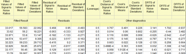
The worksheet shows how well the model predicts three Taguchi quality characteristics simultaneously: S/N ratio (robustness), mean (target performance), and standard deviation (consistency).
In addition to the fitted results and residuals in the standard DOE diagnotics, the taguchi design supports more diagnotics
Hi (Leverage)
How far a run's factor settings are from the design center. Higher values = more potential to pull the fit.
Cook's Distance
How much the fitted values change when that run is removed. Values > 1 suggest a strongly influential point
DFITS
Combines leverage and residual size to measure overall influence on the fit. A large absolute DFITS value means the run pulls the fitted surface toward itself;
Response Summary
The response summary worksheet, named DOERespondSummary, is the raw output used to compute the factor effect summaries that drive Taguchi optimization.
Static Taguchi Design
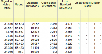
- Signal to Noise Ratios
- The S/N ratio computed for each experimental run, combining the mean response and variation into a single robustness metric. Higher = better.
- Means
- The average response value for each run (across replicates).
- Standard Deviations
- The variability of the response within each run. Lower = more consistent.
- Coefficients of Variation
- Relative variability (SD/Mean), useful for comparing spread across runs with different means.
- Ln of Standard Deviations
- Natural log transformation of SD, often used in Taguchi analysis to stabilize variance when modeling dispersion effects.
- Linear Model Design Matrix
- The coded factor settings for each run (1 = high level, –1 = low level). The leftmost column of all 1s is the intercept.
Dynamic Taguchi Design
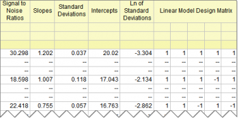
- Signal to Noise Ratios
- Dynamic S/N ratio. It rewards a strong, stable, linear signal-response relationship and penalizes scatter and non-linearity. Higher is better.
- Slopes
- The regression coefficient of response on the signal factor. This is the system's gain or sensitivity.
- Intercepts
- The baseline response when the signal factor is zero.
- Standard Deviations
- Variability around the fitted signal-response line (not around a target).
- Ln of Standard Deviations
- Log-transformed dispersion, used for modeling variance effects.
- Linear Model Design Matrix
- Coded control-factor settings (1 = high level, –1 = low level). The leading column of 1s is the intercept.