
Last Update: 10/13/2016
Assume we have two time-varying signal: Signal and Delay Signal, saved in worksheet column(B), column(D), respectively;
Assume we want to calculate the propagation delay between two signals, A model could be set up as below, f(t) is original signal while g(t) is delay signal.
=f(t-t_0)")
for all  , and
, and  is a constant.
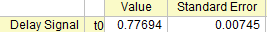
Next, we will use the Nonlinear Curve Fit to calculate the , a user defined fitting function can be constructed in this way:
The graph shown that the is approximate to 0.8, so the initial value for fitting can be set to 0.8.
| Function Name: | fitdelay |
| Function Type: | User-Defined |
| Independent Variables: | x |
| Dependent Variables: | y |
| Parameter Names: | t0 |
| Function Form: | Origin C |
| Function: |
#include <origin.h> // #include <ONLSF.H> // void _nlsffitdelay1( // Fit Parameter(s): double t0, // Independent Variable(s): double x, // Dependent Variable(s): double& y) { // Beginning of editable part NLFitContext *pCtxt = Project.GetNLFitContext(); Worksheet wks; DataRange dr; int c1,c2; dr = pCtxt->GetSourceDataRange(); //Get the source data range dr.GetRange(wks, c1, c2); //Get the source data worksheet if ( pCtxt ) { static vector vX, vY; static double nSize; BOOL bIsNewParamValues = pCtxt->IsNewParamValues(); if ( bIsNewParamValues ) { Dataset dsx(wks, 0); Dataset dsy(wks, 1); vX = dsx; vY = dsy; nSize = vY.GetSize(); } double x1; x1 = x-t0; ocmath_interpolate( &x1, &y, 1, vX, vY, nSize ); } // End of editable part } |
Please refer to this page for detailed steps about constructing user defined fitting function.
In the fitting function body, we read the response data directly from the active worksheet. So, you should perform the fit from the worksheet. Start with a new workbook and import the file \Samples\Curve Fitting\DelaySignal.dat
Keywords:Nonlinear Curve Fit, Signal Process